Compute Eigenvalues using MAPDL or SciPy

This example shows a comparison between MAPDL and Scipy eigenvalues computation power.

More specificatly, this example shows:

• How to extract the stiffness and mass matrices from a MAPDL model.

• How to use the Math module of PyMapdl to compute the first eigenvalues.

• How to can get these matrices in the SciPy world, to get the same solutions using Python resources.

• How MAPDL is really faster than SciPy :)

import math

Model setup

First load python packages we need for this example

import time

import matplotlib.pylab as plt
import numpy as np
import scipy
from scipy.sparse.linalg import eigsh

from ansys.mapdl.core import examples, launch_mapdl

Next:

• Load the ansys.mapdl module

• Get the Math module of PyMapdl

mapdl = launch_mapdl()
print(mapdl)
mm = mapdl.math

Product:             Ansys Mechanical Enterprise
MAPDL Version:       23.1
ansys.mapdl Version: 0.65.2

APDLMath EigenSolve First load the input file using MAPDL.

print(mapdl.input(examples.examples.wing_model))

/INPUT FILE=    LINE=       0
  *****MAPDL VERIFICATION RUN ONLY*****
    DO NOT USE RESULTS FOR PRODUCTION

         ***** MAPDL ANALYSIS DEFINITION (PREP7) *****

*** WARNING ***                         CP =       0.000   TIME= 00:00:00
Deactivation of element shape checking is not recommended.

*** WARNING ***                         CP =       0.000   TIME= 00:00:00
The mesh of area 1 contains PLANE42 triangles, which are much too stiff
in bending.  Use quadratic (6- or 8-node) elements if possible.

*** WARNING ***                         CP =       0.000   TIME= 00:00:00
CLEAR, SELECT, and MESH boundary condition commands are not possible
after MODMSH.


***** ROUTINE COMPLETED *****  CP =         0.000

Plot and mesh using the eplot method.

mapdl.eplot()

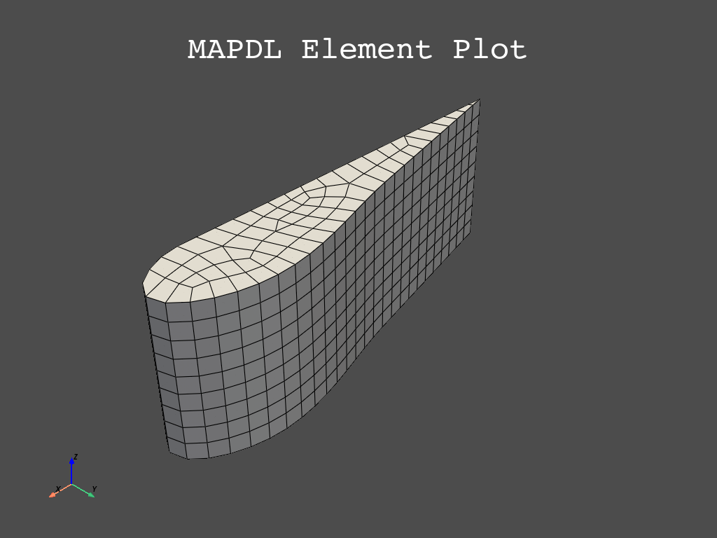
Next, setup a modal Analysis and request the $K$ and math:M matrices to be formed. MAPDL stores these matrices in a .FULL file.

print(mapdl.slashsolu())
print(mapdl.antype(antype="MODAL"))
print(mapdl.modopt(method="LANB", nmode="10", freqb="1."))
print(mapdl.wrfull(ldstep="1"))

# store the output of the solve command
output = mapdl.solve()

*****  MAPDL SOLUTION ROUTINE  *****
PERFORM A MODAL ANALYSIS
  THIS WILL BE A NEW ANALYSIS
USE SYM. BLOCK LANCZOS MODE EXTRACTION METHOD
  EXTRACT    10 MODES
  SHIFT POINT FOR EIGENVALUE CALCULATION=  1.0000
  NORMALIZE THE MODE SHAPES TO THE MASS MATRIX
STOP SOLUTION AFTER FULL FILE HAS BEEN WRITTEN
   LOADSTEP =    1 SUBSTEP =    1 EQ. ITER =    1

Matrices manipulation using PyMAPDL

Read the sparse matrices using PyMapdl.

mapdl.finish()
mm.free()
k = mm.stiff(fname="file.full")
M = mm.mass(fname="file.full")

Solve the eigenproblem using PyMapdl with APDLMath.

nev = 10
A = mm.mat(k.nrow, nev)

t1 = time.time()
ev = mm.eigs(nev, k, M, phi=A, fmin=1.0)
t2 = time.time()
mapdl_elapsed_time = t2 - t1
print("\nElapsed time to solve this problem : ", mapdl_elapsed_time)

Elapsed time to solve this problem :  0.6976687908172607

Print eigenfrequencies and accuracy.

Accuracy : $\frac{||(K-\lambda .M).\varphi |{|}_2}{||K.\varphi |{|}_2}$

mapdl_acc = np.empty(nev)

for i in range(nev):
    f = ev[i]  # Eigenfrequency (Hz)
    omega = 2 * np.pi * f  # omega = 2.pi.Frequency
    lam = omega**2  # lambda = omega^2

    phi = A[i]  # i-th eigenshape
    kphi = k.dot(phi)  # K.Phi
    mphi = M.dot(phi)  # M.Phi

    kphi_nrm = kphi.norm()  # Normalization scalar value

    mphi *= lam  # (K-\lambda.M).Phi
    kphi -= mphi

    mapdl_acc[i] = kphi.norm() / kphi_nrm  # compute the residual
    print(f"[{i}] : Freq = {f:8.2f} Hz\t Residual = {mapdl_acc[i]:.5}")

[0] : Freq =   352.39 Hz         Residual = 1.3931e-08
[1] : Freq =   385.16 Hz         Residual = 2.3293e-08
[2] : Freq =   656.78 Hz         Residual = 3.9369e-09
[3] : Freq =   764.72 Hz         Residual = 9.5144e-09
[4] : Freq =   825.33 Hz         Residual = 7.3415e-09
[5] : Freq =  1039.21 Hz         Residual = 4.9065e-09
[6] : Freq =  1143.66 Hz         Residual = 1.7584e-08
[7] : Freq =  1258.00 Hz         Residual = 5.1418e-08
[8] : Freq =  1334.23 Hz         Residual = 5.7417e-08
[9] : Freq =  1352.06 Hz         Residual = 4.1036e-08

Use SciPy to Solve the same Eigenproblem

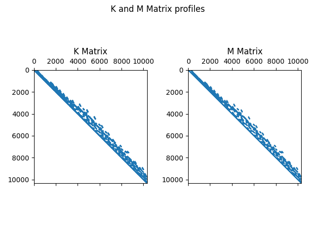
First get MAPDL sparse matrices into the Python memory as SciPy matrices.

pk = k.asarray()
pm = M.asarray()

# get_ipython().run_line_magic('matplotlib', 'inline')

fig, (ax1, ax2) = plt.subplots(1, 2)
fig.suptitle("K and M Matrix profiles")
ax1.spy(pk, markersize=0.01)
ax1.set_title("K Matrix")
ax2.spy(pm, markersize=0.01)
ax2.set_title("M Matrix")
plt.tight_layout()
plt.show(block=True)

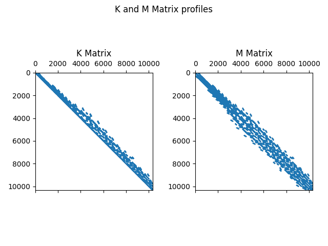
Make the sparse matrices for SciPy unsymmetric as symmetric matrices in SciPy are memory inefficient.

$K=K+K^T-diag(K)$

pkd = scipy.sparse.diags(pk.diagonal())
pK = pk + pk.transpose() - pkd
pmd = scipy.sparse.diags(pm.diagonal())
pm = pm + pm.transpose() - pmd

Plot Matrices

fig, (ax1, ax2) = plt.subplots(1, 2)
fig.suptitle("K and M Matrix profiles")
ax1.spy(pk, markersize=0.01)
ax1.set_title("K Matrix")
ax2.spy(pm, markersize=0.01)
ax2.set_title("M Matrix")
plt.tight_layout()
plt.show(block=True)

Solve the eigenproblem

t3 = time.time()
vals, vecs = eigsh(A=pK, M=pm, k=10, sigma=1, which="LA")
t4 = time.time()
scipy_elapsed_time = t4 - t3
print("\nElapsed time to solve this problem : ", scipy_elapsed_time)

Elapsed time to solve this problem :  3.766496419906616

Convert Lambda values to Frequency values: $freq=\frac{\sqrt{(}\lambda )}{2.\pi }$

freqs = np.sqrt(vals) / (2 * math.pi)

Compute the residual error for SciPy.

$Err=\frac{||(K-\lambda .M).\varphi |{|}_2}{||K.\varphi |{|}_2}$

scipy_acc = np.zeros(nev)

for i in range(nev):
    lam = vals[i]  # i-th eigenvalue
    phi = vecs.T[i]  # i-th eigenshape

    kphi = pk * phi.T  # K.Phi
    mphi = pm * phi.T  # M.Phi

    kphi_nrm = np.linalg.norm(kphi, 2)  # Normalization scalar value

    mphi *= lam  # (K-\lambda.M).Phi
    kphi -= mphi

    scipy_acc[i] = 1 - np.linalg.norm(kphi, 2) / kphi_nrm  # compute the residual
    print(f"[{i}] : Freq = {freqs[i]:8.2f} Hz\t Residual = {scipy_acc[i]:.5}")

[0] : Freq =   352.39 Hz         Residual = 8.0098e-05
[1] : Freq =   385.16 Hz         Residual = 0.00010369
[2] : Freq =   656.78 Hz         Residual = 0.00024262
[3] : Freq =   764.72 Hz         Residual = 0.00016258
[4] : Freq =   825.33 Hz         Residual = 0.00039002
[5] : Freq =  1039.21 Hz         Residual = 0.00057628
[6] : Freq =  1143.66 Hz         Residual = 0.0025916
[7] : Freq =  1258.00 Hz         Residual = 0.00033872
[8] : Freq =  1334.22 Hz         Residual = 0.00046633
[9] : Freq =  1352.06 Hz         Residual = 0.0011262

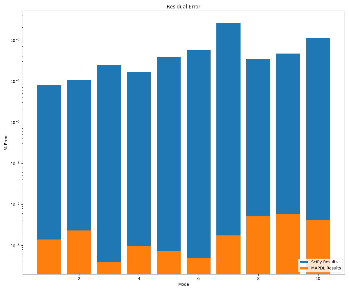
MAPDL vs Scipy comparison

MAPDL is more accurate than SciPy.

fig = plt.figure(figsize=(12, 10))
ax = plt.axes()
x = np.linspace(1, 10, 10)
plt.title("Residual Error")
plt.yscale("log")
plt.xlabel("Mode")
plt.ylabel("% Error")
ax.bar(x, scipy_acc, label="SciPy Results")
ax.bar(x, mapdl_acc, label="MAPDL Results")
plt.legend(loc="lower right")
plt.tight_layout()
plt.show()

MAPDL is faster than SciPy.

ratio = scipy_elapsed_time / mapdl_elapsed_time
print(f"Mapdl is {ratio:.3} times faster")

Mapdl is 5.4 times faster

Stop mapdl

mapdl.exit()