Build a Finite Element Model

A finite element machinery built for a quadrilateral element using an isoparametric formulation and validated with PyMAPDL.

To illustrate it with a concrete example, we take a 2D element described by the following (x, y) node locations, an isotropic material (Young’s modulus of 30e6 psi and Poission’s ratio of 0.25) and unit thickness, providing a live implementation of the discussions in Daryl Logan’s A First Course in the Finite Element Method (2nd Ed., PWS Publishing 1993).

import itertools

import matplotlib.pyplot as plt
import numpy as np

np.set_printoptions(linewidth=120)

Deriving the stiffness matrix for a 2D linear rectangular element

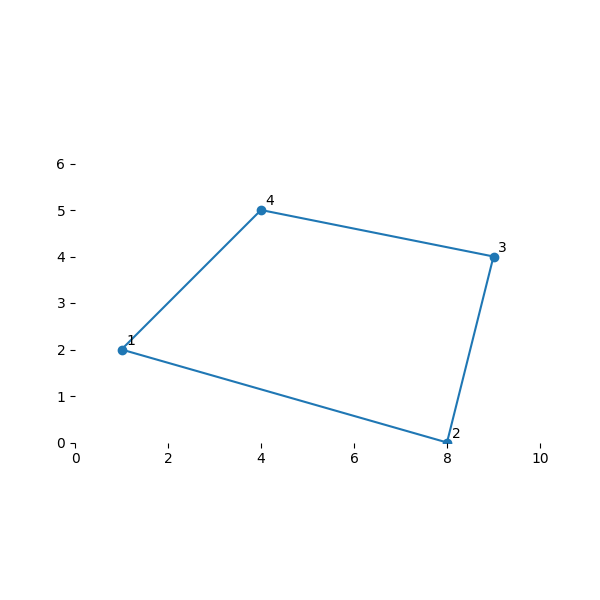
Build a basic 2D element with the following coordinates:

\[\begin{split}\begin{matrix} (1, 2) \\ (8, 0) \\ (9, 4) \\ (4, 5) \end{matrix}\end{split}\]

node_xy = [(1, 2), (8, 0), (9, 4), (4, 5)]
node_ids = list(range(1, 1 + 4))
nodes = np.array(node_xy, dtype=float)


def plot_my_mesh(nodes, points=None):
    fig = plt.figure(figsize=(6, 6))
    ax = plt.gca()
    plt.scatter(nodes[:, 0], nodes[:, 1])
    if points is not None:
        plot_pts = points if points.ndim > 1 else points[None, :]
        plt.scatter(plot_pts[:, 0], plot_pts[:, 1])
    nodes_around = np.reshape(np.take(nodes, range(10), mode="wrap"), (-1, 2))
    plt.plot(nodes_around[:, 0], nodes_around[:, 1])
    for i, n in enumerate(nodes):
        ax.annotate(i + 1, n + np.array([0.1, 0.1]))
    plt.xlim(0, 10)
    plt.ylim(0, 6)
    plt.box(False)
    ax.set_aspect(1)
    plt.show()


plot_my_mesh(nodes)

We will create an element class MyElementDemo to carry all the data and methods necessary for this demonstration. Although we could program the whole class at once (as done at the bottom of this exercise), we will add data and methods piecemeal so we can comment on their meaning. We will create an instance of this class that we’ll call my_elem to represent our specific element example

class MyElementDemo:
    def __init__(self, nodes):
        self.nodes = nodes


my_elem = MyElementDemo(nodes)

Shape Functions

Element shape functions allow us to interpolate some quantity, e.g., a component of displacement, from the corner nodes to any point throughout the element. That way, as the structure deforms, we will know not only the displacement at the nodes but also the displacements for any point within.

What’s special for an isoparametric formulation is to select a canonical shape for our 2D element. We assume that any 2D quadrilateral can be mapped to a regular square, for example a domain in \({\rm I\!R}^2\) such as \(s \in [-1,1]\) and \(t\in [-1,1]\). We derive all of our physical quantities on that square and use the mapping to transform their values for the actual shapes of our elements. This transformation will help simplify the calculation of integrals necessary for measuring how strain energy accumulates throughout the continuum of the element as the discrete nodes move and deform the shape.

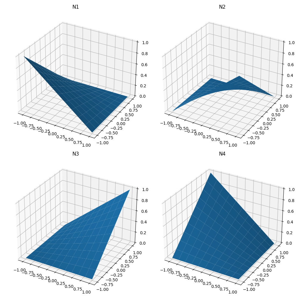
For an isoparametric 2D element, we define 4 shape functions as follows:

\[\begin{split}\begin{matrix} N_1 = \frac{(1-s)\cdot(1-t)}{4} \\ N_2 = \frac{(1+s)\cdot(1-t)}{4} \\ N_3 = \frac{(1+s)\cdot(1+t)}{4} \\ N_4 = \frac{(1-s)\cdot(1+t)}{4} \end{matrix}\end{split}\]

These functions are built in such a way that the function at node \(i\) vanishes at all other nodes and their sum is 1 at all points in the domain.

For fun, let’s plot them to see what each of them contributes to the interpolation of the element

s = np.linspace(-1, 1, 11)
t = np.linspace(-1, 1, 11)
S, T = np.meshgrid(s, t)

fig = plt.figure(figsize=(10, 10))

ax1 = fig.add_subplot(2, 2, 1, projection="3d")
ax1.plot_surface(S, T, 0.25 * (1 - S) * (1 - T))
ax1.title.set_text(r"N1")

ax2 = fig.add_subplot(2, 2, 2, projection="3d")
ax2.plot_surface(S, T, 0.25 * (1 + S) * (1 - T))
ax2.title.set_text(r"N2")

ax3 = fig.add_subplot(2, 2, 3, projection="3d")
ax3.plot_surface(S, T, 0.25 * (1 + S) * (1 + T))
ax3.title.set_text(r"N3")

ax4 = fig.add_subplot(2, 2, 4, projection="3d")
ax4.plot_surface(S, T, 0.25 * (1 - S) * (1 + T))
ax4.title.set_text(r"N4")

fig.tight_layout()
plt.show()

Let’s add the shape function method to our class

def shape_functions(self, s, t):
    return 0.25 * np.array(
        [
            (1 - s) * (1 - t),
            (1 + s) * (1 - t),
            (1 + s) * (1 + t),
            (1 - s) * (1 + t),
        ],
        dtype=float,
    )


MyElementDemo.shape_functions = shape_functions

To interpolate a quantity, e.g., position, from the nodes to arbitrary points throughout the element we use the following operation.

\[\begin{split}\begin{bmatrix} x \\ y \end{bmatrix} = \begin{bmatrix} N_{1}(s, t) & 0 & N_{2}(s, t) & 0 & N_{3}(s, t) & 0 & N_{4}(s, t) & 0 \\ 0 & N_{1}(s, t) & 0 & N_{2}(s, t) & 0 & N_{3}(s, t) & 0 & N_{4}(s, t) \end{bmatrix} \cdot \begin{bmatrix} {}^1x \\ {}^1y \\ {}^2x \\ {}^2y \\ {}^3x \\ {}^3y \\ {}^4x \\ {}^4y \end{bmatrix}\end{split}\]

\[\mathbf{X}_{\text{throughout}} = \mathbf{N} \cdot \mathbf{X}_{\text{nodal}}\]

def N(self, s, t):
    n_vec = self.shape_functions(s, t)
    return np.array(
        [
            [n_vec[0], 0, n_vec[1], 0, n_vec[2], 0, n_vec[3], 0],
            [0, n_vec[0], 0, n_vec[1], 0, n_vec[2], 0, n_vec[3]],
        ]
    )


MyElementDemo.N = N

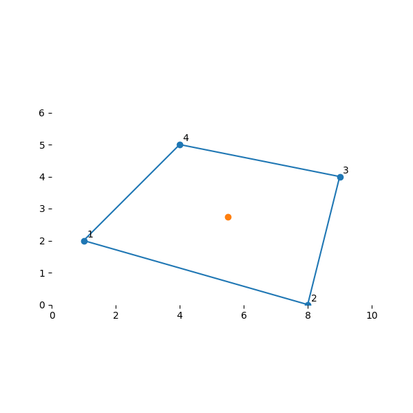
To see how this is useful, let’s interpolate some common points. The centroid of our isoparametric element was \((s,t) = (0, 0)\). Let’s see how the interpolation obtains the equivalent point in our real element:

def interpolate_nodal_values(self, s, t, nodal_values):
    return self.N(s, t).dot(nodal_values.flatten())


MyElementDemo.interpolate_nodal_values = interpolate_nodal_values

my_points = my_elem.interpolate_nodal_values(0, 0, nodes)
my_points

array([5.5 , 2.75])

Plotting the mesh.

plot_my_mesh(nodes, my_elem.interpolate_nodal_values(0, 0, nodes))

Gauss Quadrature

Gauss Quadrature is a method for approximating the integral of a function \(\int f(x) dx\) by a finite sum \(\sum w_i f(x_i)\). By sampling the function \(f(x)\) at a finite number of locations in the domain and properly scaling their values, it is possible to obtain an estimate of the integral. It turns out there are optimal locations for the sampling points \(x_i\) and their weight values \(w_i\). For a 2D function in the domain of our isoparametric element, i.e., \((s,t) \in {\rm I\!R}^2\) with \(s \in [-1,1]\) and \(t\in [-1,1]\), the optimal locations for 4 point-integration are:

gauss_pts = (
    np.array([[-1, -1], [1, -1], [1, 1], [-1, 1]], dtype=float) * 0.57735026918962
)

MyElementDemo.gauss_pts = gauss_pts
MyElementDemo.gauss_pts

array([[-0.57735027, -0.57735027],
       [ 0.57735027, -0.57735027],
       [ 0.57735027,  0.57735027],
       [-0.57735027,  0.57735027]])

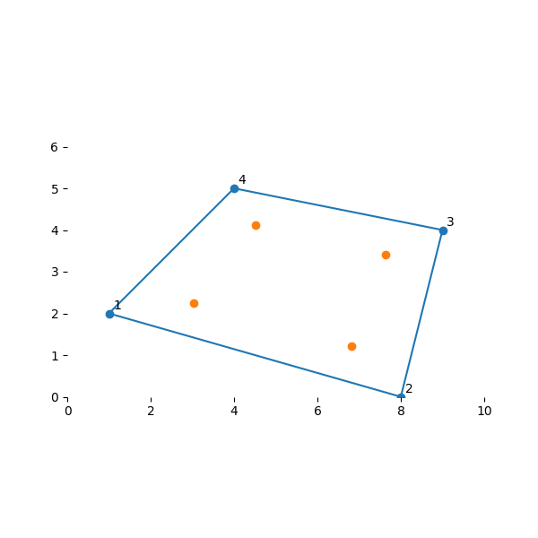
Their locations in the element of interest

gauss_pt_locs = np.stack(
    [
        my_elem.interpolate_nodal_values(*gauss_pt, nodes)
        for gauss_pt in MyElementDemo.gauss_pts
    ]
)

plot_my_mesh(nodes, gauss_pt_locs)

Strain calculation

Strain is related to displacement by a linear differential operator. For 2D, we consider only its in-plain components:

\[\begin{split}\mathbf{\varepsilon} = \begin{bmatrix} \varepsilon_x \\ \varepsilon_y \\ \gamma_{xy} \end{bmatrix} = \begin{bmatrix} \frac{\partial u_x}{\partial x} \\ \frac{\partial u_y}{\partial y} \\ \frac{\partial u_x}{\partial y} + \frac{\partial u_y}{\partial x} \end{bmatrix}\end{split}\]

and infer the operator as follows:

\[\begin{split}\begin{bmatrix} \varepsilon_x \\ \varepsilon_y \\ \gamma_{xy} \end{bmatrix} = \begin{bmatrix} \frac{\partial \left( ... \right)}{\partial x} & 0 \\ 0 & \frac{\partial \left( ... \right)}{\partial y} \\ \frac{\partial \left( ... \right)}{\partial y} & \frac{\partial \left( ... \right)}{\partial x} \end{bmatrix} \cdot \begin{bmatrix} u_x \\ u_y \end{bmatrix}\end{split}\]

We recall the displacements \(\begin{bmatrix}u_x & u_y\end{bmatrix}^T\) are known throughout the element thanks to the shape functions. Thus

\[\begin{split}\begin{bmatrix} u_x \\ u_y \end{bmatrix} = \begin{bmatrix} N_{1}(s, t) & 0 & N_{2}(s, t) & 0 & N_{3}(s, t) & 0 & N_{4}(s, t) & 0 \\ 0 & N_{1}(s, t) & 0 & N_{2}(s, t) & 0 & N_{3}(s, t) & 0 & N_{4}(s, t) \end{bmatrix} \cdot \begin{bmatrix} {}^1u_x \\ {}^1u_y \\ {}^2u_x \\ {}^2u_y \\ {}^3u_x \\ {}^3u_y \\ {}^4u_x \\ {}^4u_y \end{bmatrix}\end{split}\]

\[\mathbf{u}_{\text{throughout}} = \mathbf{N} \cdot \mathbf{u}_{\text{nodal}}\]

To incorporate the shape functions into the expressions of strain above we need to replace the differential operator relative to \(x\) and \(y\) with its equivalent expressed in terms of \(s\) and \(t\). This requires the chain rule, which in multivariate calculus is facilitated with a Jacobian matrix (and its determinant):

\[\begin{split}\begin{bmatrix} \varepsilon_x \\ \varepsilon_y \\ \gamma_{xy} \end{bmatrix} = \frac{1}{\det{\mathbf{J}}} \begin{bmatrix} \frac{\partial y}{\partial t} \frac{\partial \left( ... \right)}{\partial s} - \frac{\partial y}{\partial s} \frac{\partial \left( ... \right)}{\partial t} & 0 \\ 0 & \frac{\partial x}{\partial s} \frac{\partial \left( ... \right)}{\partial t} - \frac{\partial x}{\partial t} \frac{\partial \left( ... \right)}{\partial s} \\ \frac{\partial x}{\partial s} \frac{\partial \left( ... \right)}{\partial t} - \frac{\partial x}{\partial t} \frac{\partial \left( ... \right)}{\partial s} & \frac{\partial y}{\partial t} \frac{\partial \left( ... \right)}{\partial s} - \frac{\partial y}{\partial s} \frac{\partial \left( ... \right)}{\partial t} \end{bmatrix} \cdot \begin{bmatrix} u_x \\ u_y \end{bmatrix}\end{split}\]

\[\mathbf{\varepsilon} = \mathbf{D} \cdot \mathbf{u_{\text{throughout}}}\]

Therefore:

\[\begin{split}\begin{bmatrix} \varepsilon_x \\ \varepsilon_y \\ \gamma_{xy} \end{bmatrix} = \mathbf{D} \cdot \mathbf{N} \cdot \mathbf{u_{\text{nodal}}} = \mathbf{B} \cdot \mathbf{u_{\text{nodal}}}\end{split}\]

where

\[\begin{split}\mathbf{D}= \frac{1}{\det{\mathbf{J}}} \begin{bmatrix} \frac{\partial y}{\partial t} \frac{\partial \left( ... \right)}{\partial s} - \frac{\partial y}{\partial s} \frac{\partial \left( ... \right)}{\partial t} & 0 \\ 0 & \frac{\partial x}{\partial s} \frac{\partial \left( ... \right)}{\partial t} - \frac{\partial x}{\partial t} \frac{\partial \left( ... \right)}{\partial s} \\ \frac{\partial x}{\partial s} \frac{\partial \left( ... \right)}{\partial t} - \frac{\partial x}{\partial t} \frac{\partial \left( ... \right)}{\partial s} & \frac{\partial y}{\partial t} \frac{\partial \left( ... \right)}{\partial s} - \frac{\partial y}{\partial s} \frac{\partial \left( ... \right)}{\partial t} \end{bmatrix}\end{split}\]

and

\[\begin{split}\mathbf{J}= \begin{bmatrix} \frac{\partial x}{\partial s} & \frac{\partial y}{\partial s} \\ \frac{\partial x}{\partial t} & \frac{\partial y}{\partial t} \end{bmatrix}\end{split}\]

Implementation: Jacobians

The Jacobian can be obtained by substituting the expressions for positions \(x\) and \(y\) throughout as a function of the nodal locations with the help of the shape functions. It turns out to be equivalent to the following bilinear form:

\[\begin{split}\begin{aligned} \det{\mathbf{J}} &= \frac{1}{8} \begin{bmatrix}{}^1x & {}^2x & {}^3x & {}^4x \end{bmatrix} \cdot \begin{bmatrix} 0 & 1 - t & t-s & s-1 \\ t-1 & 0 & s+1 & -s-t \\ s-t & -s-1 & 0 & t+1 \\ 1-s & s+t & -t-1 & 0 \\ \end{bmatrix} \cdot \begin{bmatrix}{}^1y \\ {}^2y \\ {}^3y \\ {}^4y \end{bmatrix} \\&= \mathbf{X_{\text{locs}}}^T \cdot \begin{bmatrix} 0 & 1 - t & t-s & s-1 \\ t-1 & 0 & s+1 & -s-t \\ s-t & -s-1 & 0 & t+1 \\ 1-s & s+t & -t-1 & 0 \\ \end{bmatrix} \cdot \mathbf{Y_{\text{locs}}} \end{aligned}\end{split}\]

We are now ready to implement it into our element

def J(self, s, t):
    upper = np.array(
        [
            [0, -t + 1, +t - s, +s - 1],
            [0, 0, +s + 1, -s - t],
            [0, 0, 0, +t + 1],
            [0, 0, 0, 0],
        ],
        dtype=float,
    )
    temp = upper - upper.T
    return 1.0 / 8 * self.nodes[:, 0].dot(temp).dot(self.nodes[:, 1])


MyElementDemo.J = J

Next, we investigate how the Jacobians vary within the element. First for our subject element:

my_elem.J(-1, -1), my_elem.J(0, 0), my_elem.J(1, 1)

(6.75, 6.0, 5.25)

Implementation: B Matrix

Similarly, we can implement our expression for the B matrix, which converts nodal displacements \(\mathbf{u_{\text{nodal}}}\) to strains \(\mathbf{\varepsilon}\), by substituting the D operator, the shape functions and nodal locations:

\[\begin{split}\begin{bmatrix} \varepsilon_x \\ \varepsilon_y \\ \gamma_{xy} \end{bmatrix} = \mathbf{B} \cdot \mathbf{u_{\text{nodal}}}\end{split}\]

\[\mathbf{B} = \frac{1}{\det{\mathbf{J}}} \begin{bmatrix} \mathbf{B_1} & \mathbf{B_2} & \mathbf{B_3} & \mathbf{B_4} \end{bmatrix}\]

where

\[\begin{split}\mathbf{B_i} = \begin{bmatrix} a \frac{\partial N_i}{\partial s} - b \frac{\partial N_i}{\partial t} & 0 \\ 0 & c \frac{\partial N_i}{\partial t} - d \frac{\partial N_i}{\partial s} \\ c \frac{\partial N_i}{\partial t} - d \frac{\partial N_i}{\partial s} & a \frac{\partial N_i}{\partial s} - b \frac{\partial N_i}{\partial t} \end{bmatrix}\end{split}\]

and

\[\begin{split}\begin{bmatrix} d & c\\ a & b \end{bmatrix}= \frac{1}{4} \begin{bmatrix} \mathbf{X_{\text{locs}}}^T \\ \mathbf{Y_{\text{locs}}}^T \end{bmatrix} \cdot \begin{bmatrix} \mathbf{S} & \mathbf{T} \end{bmatrix}\end{split}\]

for

\[\begin{split}\mathbf{S} = \begin{bmatrix} s - 1 \\ -(s+1) \\ s+1 \\ -(s-1) \end{bmatrix}\end{split}\]

\[\begin{split}\mathbf{T} = \begin{bmatrix} t - 1 \\ -(t-1) \\ t+1 \\ -(s+1) \end{bmatrix}\end{split}\]

def grad_N(self, s, t):
    return 0.25 * np.array(
        [
            [-(1 - t), +(1 - t), +(1 + t), -(1 + t)],
            [-(1 - s), -(1 + s), +(1 + s), +(1 - s)],
        ],
        dtype=float,
    )


def B(self, s, t):
    j = self.J(s, t)
    S = np.array([-1 + s, -1 - s, +1 + s, +1 - s], dtype=float)
    T = np.array([-1 + t, +1 - t, +1 + t, -1 - t], dtype=float)
    [d, c], [a, b] = (
        0.25 * np.c_[self.nodes[:, 0], self.nodes[:, 1]].T.dot(np.c_[S, T])
    ).tolist()
    n = self.grad_N(s, t)

    def _bi_(i):
        return np.array(
            [
                [a * n[0, i] - b * n[1, i], 0],
                [0, c * n[1, i] - d * n[0, i]],
                [c * n[1, i] - d * n[0, i], a * n[0, i] - b * n[1, i]],
            ],
            dtype=float,
        )

    return 1.0 / j * np.c_[_bi_(0), _bi_(1), _bi_(2), _bi_(3)]


MyElementDemo.grad_N = grad_N
MyElementDemo.B = B

my_elem.B(0, 0)

array([[-0.10416667,  0.        ,  0.04166667,  0.        ,  0.10416667,  0.        , -0.04166667,  0.        ],
       [ 0.        , -0.08333333,  0.        , -0.16666667,  0.        ,  0.08333333,  0.        ,  0.16666667],
       [-0.08333333, -0.10416667, -0.16666667,  0.04166667,  0.08333333,  0.10416667,  0.16666667, -0.04166667]])

Stress Calculation

The leap from strains to stresses involves the constitutive model, i.e., the material properties. This demo assumes a very simple case, i.e., a linear isotropic material which converts strains to stresses according to the following matrix:

\[\mathbf{\sigma} = \mathbf{C} \cdot \mathbf{\varepsilon}\]

\[\begin{split}\begin{bmatrix} \sigma_x \\ \sigma_y \\ \tau_{xy} \end{bmatrix} = \begin{bmatrix} 1 & \nu & 0 \\ \nu & 1 & 0 \\ 0 & 0 & 1 \end{bmatrix} \begin{bmatrix} \varepsilon_x \\ \varepsilon_y \\ \gamma_{xy} \end{bmatrix}\end{split}\]

class Isotropic:
    def __init__(self, ex, nu):
        self.nu = nu
        self.ex = ex

    def evaluate(self):
        d = np.array(
            [[1, self.nu, 0], [self.nu, 1, 0], [0, 0, (1 - self.nu) / 2.0]],
            dtype=float,
        )

        return d * (self.ex / (1 - self.nu**2))


isotropic = Isotropic(30e6, 0.25)

Stiffness Calculation

The total energy of a system \(E\), comprising an element on which nodal forces \(\mathbf{F}_{\text{nodal}}\) are applied and undergoes nodal deformation \(\mathbf{u}_{\text{nodal}}\) is:

\[E = - \mathbf{F}_{\text{nodal}} \cdot \mathbf{u}_{\text{nodal}} + \frac{1}{2} \iiint_V{} \mathbf{\varepsilon}^T \cdot \mathbf{\sigma} \,dV\]

The first term stems from the work by the force at the nodes while the second measures the strain energy density accumulated throughout the element volume as it deforms.

As we saw, both stress and strain relate back to the nodal displacements through the B (courtesy of the shape functions), i.e., \(\mathbf{\varepsilon} = \mathbf{B} \cdot \mathbf{u}_{\text{nodal}}\) and \(\mathbf{\sigma} = \mathbf{C} \cdot \mathbf{B} \cdot \mathbf{u}_{\text{nodal}}\) thus:

\[E = -\mathbf{F}_{\text{nodal}} \cdot \mathbf{u}_{\text{nodal}} + \frac{1}{2} \iiint_V{} \mathbf{u}_{\text{nodal}}^T \cdot \mathbf{B}^T \cdot \mathbf{C} \cdot \mathbf{B} \cdot \mathbf{u}_{\text{nodal}} \,dV\]

Our assumed linear shape functions are not as rich as the true functions governing the actual deformation of the structure in real life. Imagine a Taylor expansion: our linear shape function captures up to the first polynomial term, whereas the true shape function could have arbitrarily many beyond that. One way this shows up is in the total energy of our system. When constrained to use our limited fidelity shape functions the system will accumulate a higher total energy than that of the true solution it is meant to approximate. To seek the best approximation, it makes sense to find a minimum of this total energy relative to the possible solutions, i.e., nodal displacements \(\mathbf{u}_{\text{nodal}}\). Loyal to our calculus roots, we look for the minimum by taking the corresponding partial derivative:

\[\frac{\partial E}{\partial \mathbf{u}_{\text{nodal}}} = -\mathbf{F}_{\text{nodal}} + \frac{1}{2} \iiint_V{} \mathbf{B}^T \cdot \mathbf{C} \cdot \mathbf{B} \cdot \mathbf{u}_{\text{nodal}} \,dV =0\]

\[\mathbf{F}_{\text{nodal}} = \frac{1}{2} \iiint_V{} \mathbf{B}^T \cdot \mathbf{C} \cdot \mathbf{B} \cdot \mathbf{u}_{\text{nodal}} \,dV = \mathbf{K} \cdot \mathbf{u}_{\text{nodal}}\]

Thus, we’ve unlocked the Hooke’s law stiffness hidden in the integral:

\[\mathbf{K} = \iiint_V{} \mathbf{B}^T \cdot \mathbf{C} \cdot \mathbf{B} \,dV\]

For our planar element, assumed to have constant thickness \(h\) and area \(A\):

\[\mathbf{K} = h \iint_A{} \mathbf{B}^T \cdot \mathbf{C} \cdot \mathbf{B} \,dA=h \iint_A{} \mathbf{B}^T \cdot \mathbf{C} \cdot \mathbf{B} \,dx \,dy = h \iint_A{} \mathbf{B}^T \cdot \mathbf{C} \cdot \mathbf{B} \cdot \det(\mathbf{J}) \,ds \,dt\]

And the integral can be approximated by Gaussian quadrature through a weighted sum with the optimal sampling points for \(\mathbf{B}\):

\[\mathbf{K}\approx h \sum_{(s,t) \in \text{Gauss}} w(s,t) \cdot \mathbf{B}^T(s,t) \cdot \mathbf{C} \cdot \mathbf{B}(s,t) \cdot \det(\mathbf{J}(s,t))\]

Thus the use of an isoparametric formulation allowed us to make this integration easy, since the domain of integration is constant, regardless of the shape of the 2D quadrilateral at hand.

def K(self, C):
    tot = np.zeros((self.ndof, self.ndof), dtype=float)
    for st in self.gauss_pts:
        B = self.B(*(st.tolist()))
        J = self.J(*(st.tolist()))
        tot += B.T.dot(C).dot(B) * J

    return tot


MyElementDemo.K = K
MyElementDemo.ndof = 8

stiffness = my_elem.K(isotropic.evaluate())
print(stiffness)

[[ 12875125.32026284   4266737.21733318  -1512012.17927291   2247558.57561918  -7065315.06442397  -4038004.53009543
   -4297798.07656597  -2476291.26285693]
 [  4266737.21733318  12388604.21076075   4247558.57561918   6047863.05744317  -4038004.53009543  -3405127.91949808
   -4476291.26285693 -15031339.34870584]
 [ -1512012.17927291   4247558.57561918  11200772.34413869  -3259812.11243548  -3467825.1828747   -4443615.16468011
   -6220934.98199108   3455868.70149641]
 [  2247558.57561918   6047863.05744316  -3259812.11243548  24720879.28409633  -2443615.16468011 -13747985.59281117
    3455868.70149641 -17020756.74872833]
 [ -7065315.06442397  -4038004.53009543  -3467825.1828747   -2443615.16468011  14535071.10764538   4332089.41368683
   -4001930.86034672   2149530.28108871]
 [ -4038004.53009543  -3405127.91949808  -4443615.16468011 -13747985.59281117   4332089.41368683  14955311.72255009
    4149530.28108871   2197801.78975916]
 [ -4297798.07656596  -4476291.26285693  -6220934.98199108   3455868.70149641  -4001930.86034672   4149530.28108871
   14520663.91890376  -3129107.7197282 ]
 [ -2476291.26285693 -15031339.34870584   3455868.70149641 -17020756.74872833   2149530.28108871   2197801.78975916
   -3129107.7197282   29854294.307675  ]]

stiffness_scaled = np.round(stiffness / 1e4)
print(stiffness_scaled)

[[ 1288.   427.  -151.   225.  -707.  -404.  -430.  -248.]
 [  427.  1239.   425.   605.  -404.  -341.  -448. -1503.]
 [ -151.   425.  1120.  -326.  -347.  -444.  -622.   346.]
 [  225.   605.  -326.  2472.  -244. -1375.   346. -1702.]
 [ -707.  -404.  -347.  -244.  1454.   433.  -400.   215.]
 [ -404.  -341.  -444. -1375.   433.  1496.   415.   220.]
 [ -430.  -448.  -622.   346.  -400.   415.  1452.  -313.]
 [ -248. -1503.   346. -1702.   215.   220.  -313.  2985.]]

Putting it all together

Creating Elem2D class.

class Elem2D:
    gauss_pts = (
        np.array([[-1, -1], [1, -1], [1, 1], [-1, 1]], dtype=float) * 0.57735026918962
    )
    nnodes = 4
    ndof = 8

    def __init__(self, nodes):
        self.nodes = nodes

    def B(self, s, t):
        j = self.J(s, t)
        S = np.array([-1 + s, -1 - s, +1 + s, +1 - s], dtype=float)
        T = np.array([-1 + t, +1 - t, +1 + t, -1 - t], dtype=float)
        [d, c], [a, b] = (
            0.25 * np.c_[self.nodes[:, 0], self.nodes[:, 1]].T.dot(np.c_[S, T])
        ).tolist()
        n = self.__grad_Ni(s, t)

        def _bi_(i):
            return np.array(
                [
                    [a * n[0, i] - b * n[1, i], 0],
                    [0, c * n[1, i] - d * n[0, i]],
                    [c * n[1, i] - d * n[0, i], a * n[0, i] - b * n[1, i]],
                ],
                dtype=float,
            )

        return 1.0 / j * np.c_[_bi_(0), _bi_(1), _bi_(2), _bi_(3)]

    def __Ni(self, s, t):
        return 0.25 * np.array(
            [
                (1 - s) * (1 - t),
                (1 + s) * (1 - t),
                (1 + s) * (1 + t),
                (1 - s) * (1 + t),
            ],
            dtype=float,
        )

    def __grad_Ni(self, s, t):
        return 0.25 * np.array(
            [
                [-(1 - t), +(1 - t), +(1 + t), -(1 + t)],
                [-(1 - s), -(1 + s), +(1 + s), +(1 - s)],
            ],
            dtype=float,
        )

    def J(self, s, t):
        upper = np.array(
            [
                [0, -t + 1, +t - s, +s - 1],
                [0, 0, +s + 1, -s - t],
                [0, 0, 0, +t + 1],
                [0, 0, 0, 0],
            ],
            dtype=float,
        )
        temp = upper - upper.T
        return 1.0 / 8 * self.nodes[:, 0].dot(temp).dot(self.nodes[:, 1])

    def k(self, C):
        tot = np.zeros((self.ndof, self.ndof), dtype=float)
        for st in self.gauss_pts:
            B = self.B(*(st.tolist()))
            J = self.J(*(st.tolist()))
            tot += B.T.dot(C).dot(B) * J

        return tot

    def N(self, s, t):
        n_vec = self.___Ni(s, t)
        return np.array(
            [
                [n_vec[0], 0, n_vec[1], 0, n_vec[2], 0, n_vec[3], 0],
                [0, n_vec[0], 0, n_vec[1], 0, n_vec[2], 0, n_vec[3]],
            ]
        )

    def M(self, rho):
        tot = np.zeros((8, 8), dtype=float)
        for st in self.gauss_pts:
            n_array = self.N(*(st.tolist()))
            tot += n_array.T.dot(n_array)

        return tot

Isotropic class definition

class Isotropic:
    def __init__(self, ex, nu):
        self.nu = nu
        self.ex = ex

    def evaluate(self):
        d = np.array(
            [[1, self.nu, 0], [self.nu, 1, 0], [0, 0, (1 - self.nu) / 2.0]],
            dtype=float,
        )

        return d * (self.ex / (1 - self.nu**2))

Applying the created classes.

isotropic = Isotropic(30e6, 0.25)
elem = Elem2D(nodes)

stiffness = elem.k(isotropic.evaluate())

stiffness_scaled = np.round(stiffness / 1e4)
print(stiffness_scaled)

[[ 1288.   427.  -151.   225.  -707.  -404.  -430.  -248.]
 [  427.  1239.   425.   605.  -404.  -341.  -448. -1503.]
 [ -151.   425.  1120.  -326.  -347.  -444.  -622.   346.]
 [  225.   605.  -326.  2472.  -244. -1375.   346. -1702.]
 [ -707.  -404.  -347.  -244.  1454.   433.  -400.   215.]
 [ -404.  -341.  -444. -1375.   433.  1496.   415.   220.]
 [ -430.  -448.  -622.   346.  -400.   415.  1452.  -313.]
 [ -248. -1503.   346. -1702.   215.   220.  -313.  2985.]]

Element in PyMAPDL

Now let’s obtain the same stiffness matrix from MAPDL

launch PyMAPDL

from ansys.mapdl.core import launch_mapdl

mapdl = launch_mapdl()
mapdl.clear()

Create a use a 2-D 4-Node Structural Solid element with matching material properties.

mapdl.prep7()
mapdl.et(1, 182)
mapdl.mp("ex", 1, 30e6)  # Young's modulus
mapdl.mp("nuxy", 1, 0.25)  # Poisson's ratio
mapdl.mp("dens", 1, 1)
# unit density

MATERIAL          1     DENS =   1.000000

Create the nodes at the same locations as above.

for i, n in zip(node_ids, nodes):
    mapdl.n(i, *n)

Setup our element with the corresponding material properties.

_ = mapdl.e(*node_ids)  # Using '_ =' to hide output.

Setup the static analysis.

mapdl.slashsolu()
mapdl.antype("static", "new")

PERFORM A STATIC ANALYSIS
  THIS WILL BE A NEW ANALYSIS

Solve and permit one degree of freedom of each mode to be free per solution.

dof_list = list(itertools.product(node_ids, ["ux", "uy"]))

for node_id, dof in dof_list:
    mapdl.d("all", "all")
    mapdl.d(node_id, dof, 1)
    mapdl.solve()

mapdl.finish()

FINISH SOLUTION PROCESSING

 *** NOTE ***                            CP =       0.000   TIME= 00:00:00
 Distributed parallel processing has been reactivated.


 ***** ROUTINE COMPLETED *****  CP =         0.000

The columns of the stiffness matrix appear as nodal force reactions

results = []

for i, _ in enumerate(dof_list):
    mapdl.post1()
    mapdl.set(i + 1)
    prrsol_f = mapdl.prrsol("f").to_array()[:, 1:]  # Omitting node column (0)
    results.append(prrsol_f)

for txt in results:
    print(txt)
    print("=" * 80)

[[12875000.  4266700.]
 [-1512000.  2247600.]
 [-7065300. -4038000.]
 [-4297800. -2476300.]]
================================================================================
[[  4266700.  12389000.]
 [  4247600.   6047900.]
 [ -4038000.  -3405100.]
 [ -4476300. -15031000.]]
================================================================================
[[-1512000.  4247600.]
 [11201000. -3259800.]
 [-3467800. -4443600.]
 [-6220900.  3455900.]]
================================================================================
[[  2247600.   6047900.]
 [ -3259800.  24721000.]
 [ -2443600. -13748000.]
 [  3455900. -17021000.]]
================================================================================
[[-7065300. -4038000.]
 [-3467800. -2443600.]
 [14535000.  4332100.]
 [-4001900.  2149500.]]
================================================================================
[[ -4038000.  -3405100.]
 [ -4443600. -13748000.]
 [  4332100.  14955000.]
 [  4149500.   2197800.]]
================================================================================
[[-4297800. -4476300.]
 [-6220900.  3455900.]
 [-4001900.  4149500.]
 [14521000. -3129100.]]
================================================================================
[[ -2476300. -15031000.]
 [  3455900. -17021000.]
 [  2149500.   2197800.]
 [ -3129100.  29854000.]]
================================================================================

Now, apply this to the whole matrix and output it.

stiffness_mapdl = np.array(results)
stiffness_mapdl = stiffness_mapdl.reshape(8, 8)
stiffnes_mapdl_scaled = np.round(stiffness_mapdl / 1e4)
print(stiffnes_mapdl_scaled)

[[ 1288.   427.  -151.   225.  -707.  -404.  -430.  -248.]
 [  427.  1239.   425.   605.  -404.  -341.  -448. -1503.]
 [ -151.   425.  1120.  -326.  -347.  -444.  -622.   346.]
 [  225.   605.  -326.  2472.  -244. -1375.   346. -1702.]
 [ -707.  -404.  -347.  -244.  1454.   433.  -400.   215.]
 [ -404.  -341.  -444. -1375.   433.  1496.   415.   220.]
 [ -430.  -448.  -622.   346.  -400.   415.  1452.  -313.]
 [ -248. -1503.   346. -1702.   215.   220.  -313.  2985.]]

Which is identical to the stiffness matrix obtained from our academic formulation.

print(stiffness_scaled)

[[ 1288.   427.  -151.   225.  -707.  -404.  -430.  -248.]
 [  427.  1239.   425.   605.  -404.  -341.  -448. -1503.]
 [ -151.   425.  1120.  -326.  -347.  -444.  -622.   346.]
 [  225.   605.  -326.  2472.  -244. -1375.   346. -1702.]
 [ -707.  -404.  -347.  -244.  1454.   433.  -400.   215.]
 [ -404.  -341.  -444. -1375.   433.  1496.   415.   220.]
 [ -430.  -448.  -622.   346.  -400.   415.  1452.  -313.]
 [ -248. -1503.   346. -1702.   215.   220.  -313.  2985.]]

Show that the stiffness matrix in MAPDL matches what we derived.

if np.allclose(stiffnes_mapdl_scaled, stiffness_scaled):
    print("Both matrices are the equal within tolerance.")

Both matrices are the equal within tolerance.

Stop mapdl

mapdl.exit()