Create your own Python command-line app#

This example shows how to create your own command-line app in Python that uses PyMAPDL to perform some simulations. This usage is quite convenient when automating workflows. You can build different PyMAPDL apps that can be called from the command line with different arguments.

Simulation configuration#

The rotor.py script implements a command-line interface for calculating the first natural frequency of a simplified rotor with a given number of blades and a specific material configuration.

# Script to calculate the first natural frequecy of
# a rotor for a given set of properties

# Import packages
import numpy as np

from ansys.mapdl.core import launch_mapdl

# Launch MAPDL
mapdl = launch_mapdl(port=50052)
mapdl.clear()
mapdl.prep7()

# Define input properties
n_blades = 8
blade_length = 0.2

elastic_modulus = 200e9  # N/m2
density = 7850  # kg/m3

# Define other properties
center_radious = 0.1
blade_thickness = 0.02
section_length = 0.06

## Define material
# Material 1: Steel
mapdl.mp("NUXY", 1, 0.31)
mapdl.mp("DENS", 1, density)
mapdl.mp("EX", 1, elastic_modulus)

## Geometry
# Plot center
area_cyl = mapdl.cyl4(0, 0, center_radious)

# Define path for dragging
k0 = mapdl.k(x=0, y=0, z=0)
k1 = mapdl.k(x=0, y=0, z=section_length)

line_path = mapdl.l(k0, k1)

mapdl.vdrag(area_cyl, nlp1=line_path)
center_vol = mapdl.geometry.vnum[0]

# Create spline
precision = 5
advance = section_length / precision

spline = []
for i in range(precision + 1):
    if i != 0:
        k0 = mapdl.k("", x_, y_, z_)
    angle_ = i * (360 / n_blades) / precision
    x_ = section_length * np.cos(np.deg2rad(angle_))
    y_ = section_length * np.sin(np.deg2rad(angle_))
    z_ = i * advance

    if i != 0:
        k1 = mapdl.k("", x_, y_, z_)
        spline.append(mapdl.l(k0, k1))

# Merge lines
mapdl.nummrg("kp")

# Create area of the blade
point_0 = mapdl.k("", center_radious * 0.6, -blade_thickness / 2, 0)
point_1 = mapdl.k("", center_radious + blade_length, -blade_thickness / 2, 0)
point_2 = mapdl.k("", center_radious + blade_length, blade_thickness / 2, 0)
point_3 = mapdl.k("", center_radious, blade_thickness / 2, 0)
blade_area = mapdl.a(point_0, point_1, point_2, point_3)

# Drag area to
mapdl.vdrag(
    blade_area,
    nlp1=spline[0],
    nlp2=spline[1],
    nlp3=spline[2],
    nlp4=spline[3],
    nlp5=spline[4],
)


# Glue blades
mapdl.allsel()
mapdl.vsel("u", vmin=center_vol)
mapdl.vadd("all")
blade_volu = mapdl.geometry.vnum[0]

# Define cutting blade and circle
mapdl.allsel()
mapdl.vsbv(blade_volu, center_vol, keep2="keep")
blade_volu = mapdl.geometry.vnum[-1]

# Define symmetry
mapdl.csys(1)  # switch to cylindrical
mapdl.vgen(n_blades, blade_volu, dy=360 / n_blades, imove=0)
mapdl.csys(0)  # switch to global coordinate system

# Glue/add volumes
mapdl.allsel()
mapdl.vadd("all")
center_vol = mapdl.geometry.vnum[-1]

# Mesh
mapdl.allsel()
mapdl.et(1, "SOLID186")
mapdl.esize(blade_thickness / 2)
mapdl.mshape(1, "3D")
mapdl.vmesh("all")

# Apply loads
mapdl.nsel("all")
mapdl.nsel("r", "loc", "z", 0)
mapdl.csys(1)
mapdl.nsel("r", "loc", "x", 0, center_radious)
mapdl.d("all", "ux", 0)
mapdl.d("all", "uy", 0)
mapdl.d("all", "uz", 0)
mapdl.csys(0)

# Solve
mapdl.allsel()
mapdl.nummrg("all")
mapdl.slashsolu()
nmodes = 10  # Get the first 10 modes
output = mapdl.modal_analysis(nmode=nmodes)

# Postprocessing
mapdl.post1()
modes = mapdl.set("list").to_array()
freqs = modes[:, 1]

# Output values
first_frequency = freqs[0]
print(f"The first natural frequency is {first_frequency} Hz.")

Convert a script to a Python app#

To use the preceding script from a terminal, you must convert it to a Python app. In this case, the app uses a command-line interface to provide the options to PyMAPDL.

To specify the options, the package Click is used. Another suitable package is the builtin package argparse.

First, you must convert the script to a function. You can accomplish this by using the input arguments in a function signature.

In this case, the following arguments must be specified:

n_blades: Number of blades.
blade_length: Length of each blade.
elastic_modulus: Elastic modulus of the material.
density: Density of the material.

You can then define the function like this:

# Import packages
import numpy as np

from ansys.mapdl.core import launch_mapdl
def main(n_blades, blade_length, elastic_modulus, density):
    print(
        "Initialize script with values:\n"
        f"Number of blades: {n_blades}\nBlade length: {blade_length} m\n"
        f"Elastic modulus: {elastic_modulus/1E9} GPa\nDensity: {density} Kg/m3"
    )

You introduce the values of these parameters by adding this code immediately before the function definition:

import click

@click.command()
@click.argument(
    "n_blades",
)  # arguments are mandatory
@click.option("--blade_length", default=0.2, help="Length of each blade.")  # optionals
@click.option(
    "--elastic_modulus", default=200e9, help="Elastic modulus of the material."
)
@click.option("--density", default=7850, help="Density of the material.")
def main(n_blades, blade_length, elastic_modulus, density):
    print(
        "Initialize script with values:\n"
        f"Number of blades: {n_blades}\nBlade length: {blade_length} m\n"
        f"Elastic modulus: {elastic_modulus/1E9} GPa\nDensity: {density} Kg/m3"
    )
    # Launch MAPDL

Warning

Because the Click package uses decorators (@click.XXX, you must specify Click commands immediately before the function definition.

In addition, you must add the call to the newly created function at the end of the script:

if __name__ == "__main__":
    main()

This ensure the new function is called when the script is executed.

Now you can call your function from the command line using this code:

$ python rotor.py 8
Initialize script with values:
Number of blades: 8
Blade length: 0.2 m
Elastic modulus: 200.0 GPa
Density: 7850 Kg/m3
Solving...
The first natural frequency is 325.11 Hz.

The preceding code sets the number of blades to 8. This code shows how you can input other arguments:

$ python rotor.py 8 --density 7000
Initialize script with values:
Number of blades: 8
Blade length: 0.2 m
Elastic modulus: 200.0 GPa
Density: 7000 Kg/m3
Solving...
The first natural frequency is 344.28 Hz.

Advanced usage#

You can use these concepts to make Python create files with specific results that you can later use in other apps.

Postprocess images using ImageMagick#

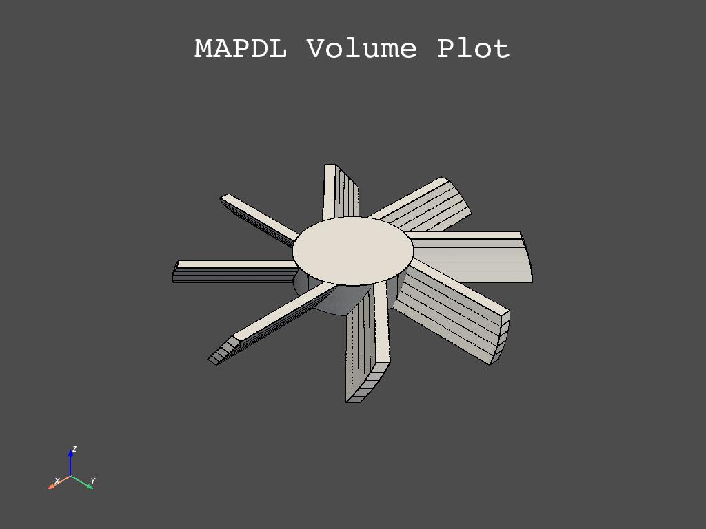
To create an image with PyMAPDL, you can add this code to the rotor.py file:

mapdl.vplot(savefig="volumes.jpg")

To add a frame, you can use ImageMagick:

mogrify -mattecolor \#f1ce80 -frame 10x10 volumes.jpg

You can also use Imagemagick to add a watermark:

COMPOSITE=/usr/bin/composite
$COMPOSITE -gravity SouthEast watermark.jpg volumes.jpg volumes_with_watermark.jpg

Here are descriptions for values used in the preceding code:

-gravity: Location of the watermark in case the watermark is smaller than the image.
COMPOSITE: Path to the ImageMagick composite function.
watermark.png: Name of the PNG file with the watermark image.
volumes_with_watermark.jpg: Name of the JPG file to save the output to.

The final results should look like the ones in this image:

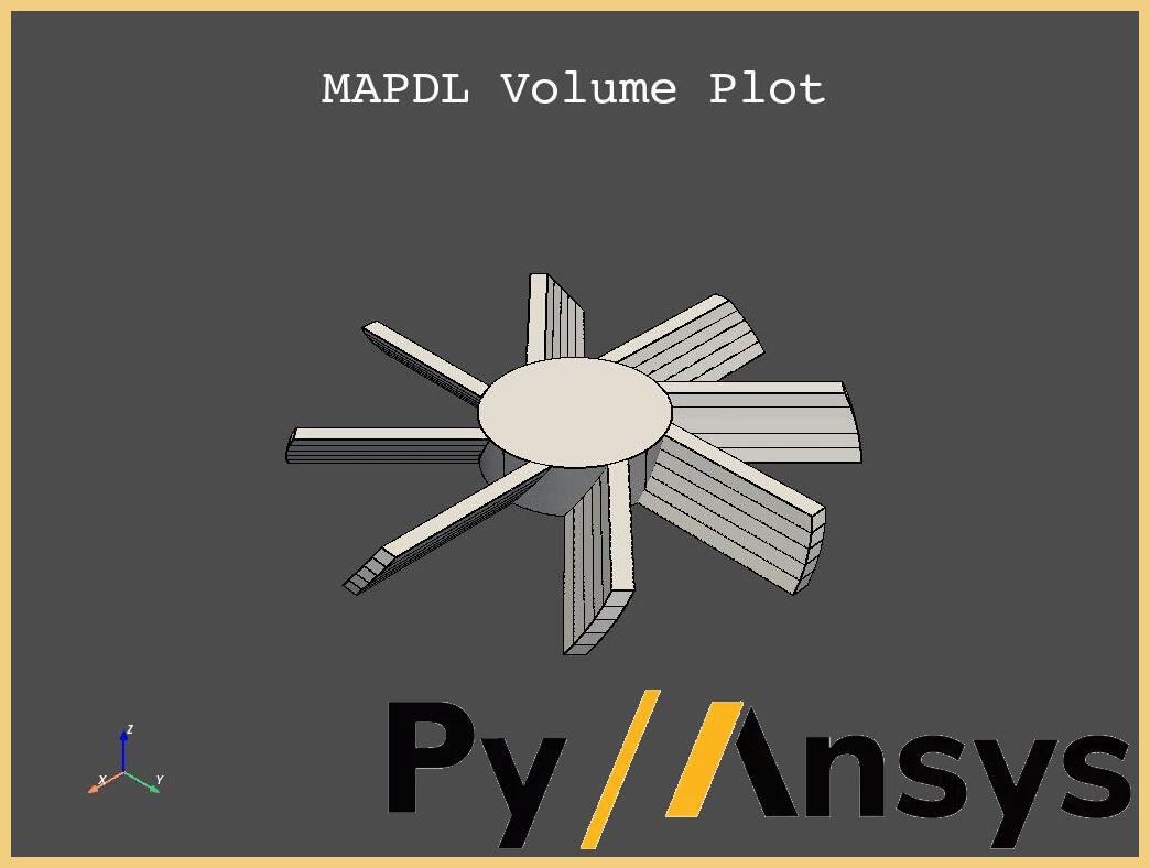
../../../_images/volumes_with_watermark.jpg — Volumes image with watermark#

Usage on the cloud#

Using these concepts, you can deploy your own apps to the cloud.

For example, you can execute the previous example on a GitHub runner using this approach (non-tested):

my_job:
   name: 'Generate watermarked images'
   runs-on: ubuntu-latest

   steps:
      - name: "Install Git and check out project"
        uses: actions/checkout@v3

      - name: "Set up Python"
        uses: actions/setup-python@v4

      - name: "Install ansys-mapdl-core"
        run: |
            python -m pip install ansys-mapdl-core

      - name: "Install ImageMagic"
        run: |
         sudo apt install imagemagick

      - name: "Generate images with PyMAPDL"
        run: |
         python rotor.py 4 --density 7000

      - name: "Postprocess images"
        run: |
           COMPOSITE=/usr/bin/composite
           mogrify -mattecolor #f1ce80 -frame 10x10 volume.jpg
           $COMPOSITE -gravity SouthEast watermark.jpg volumes.jpg volumes_with_watermark.jpg

Additional files#

You can use these links to download the example files:

Original rotor.py script
App cli_rotor.py script