Create your own Python command-line app#
This example shows how to create your own command-line app in Python that uses PyMAPDL to perform some simulations. This usage is quite convenient when automating workflows. You can build different PyMAPDL apps that can be called from the command line with different arguments.
Simulation configuration#
The rotor.py script implements a
command-line interface for calculating the first
natural frequency of a simplified rotor with a given number of
blades and a specific material configuration.
# Copyright (C) 2016 - 2026 ANSYS, Inc. and/or its affiliates.
# SPDX-License-Identifier: MIT
#
#
# Permission is hereby granted, free of charge, to any person obtaining a copy
# of this software and associated documentation files (the "Software"), to deal
# in the Software without restriction, including without limitation the rights
# to use, copy, modify, merge, publish, distribute, sublicense, and/or sell
# copies of the Software, and to permit persons to whom the Software is
# furnished to do so, subject to the following conditions:
#
# The above copyright notice and this permission notice shall be included in all
# copies or substantial portions of the Software.
#
# THE SOFTWARE IS PROVIDED "AS IS", WITHOUT WARRANTY OF ANY KIND, EXPRESS OR
# IMPLIED, INCLUDING BUT NOT LIMITED TO THE WARRANTIES OF MERCHANTABILITY,
# FITNESS FOR A PARTICULAR PURPOSE AND NONINFRINGEMENT. IN NO EVENT SHALL THE
# AUTHORS OR COPYRIGHT HOLDERS BE LIABLE FOR ANY CLAIM, DAMAGES OR OTHER
# LIABILITY, WHETHER IN AN ACTION OF CONTRACT, TORT OR OTHERWISE, ARISING FROM,
# OUT OF OR IN CONNECTION WITH THE SOFTWARE OR THE USE OR OTHER DEALINGS IN THE
# SOFTWARE.

# Script to calculate the first natural frequency of a rotor for a given set of
# properties

# Import packages
import numpy as np

from ansys.mapdl.core import launch_mapdl

# Launch MAPDL
mapdl = launch_mapdl()
mapdl.clear()
mapdl.prep7()

# Define input properties
n_blades = 8
blade_length = 0.2

elastic_modulus = 200e9  # N/m2
density = 7850  # kg/m3

# Define other properties
center_radious = 0.1
blade_thickness = 0.02
section_length = 0.06

## Define material
# Material 1: Steel
mapdl.mp("NUXY", 1, 0.31)
mapdl.mp("DENS", 1, density)
mapdl.mp("EX", 1, elastic_modulus)

## Geometry
# Plot center
area_cyl = mapdl.cyl4(0, 0, center_radious)

# Define path for dragging
k0 = mapdl.k(x=0, y=0, z=0)
k1 = mapdl.k(x=0, y=0, z=section_length)

line_path = mapdl.l(k0, k1)

mapdl.vdrag(area_cyl, nlp1=line_path)
center_vol = mapdl.geometry.vnum[0]

# Create spline
precision = 5
advance = section_length / precision

spline = []
for i in range(precision + 1):
    if i != 0:
        k0 = mapdl.k("", x_, y_, z_)
    angle_ = i * (360 / n_blades) / precision
    x_ = section_length * np.cos(np.deg2rad(angle_))
    y_ = section_length * np.sin(np.deg2rad(angle_))
    z_ = i * advance

    if i != 0:
        k1 = mapdl.k("", x_, y_, z_)
        spline.append(mapdl.l(k0, k1))

# Merge lines
mapdl.nummrg("kp")

# Create area of the blade
point_0 = mapdl.k("", center_radious * 0.6, -blade_thickness / 2, 0)
point_1 = mapdl.k("", center_radious + blade_length, -blade_thickness / 2, 0)
point_2 = mapdl.k("", center_radious + blade_length, blade_thickness / 2, 0)
point_3 = mapdl.k("", center_radious, blade_thickness / 2, 0)
blade_area = mapdl.a(point_0, point_1, point_2, point_3)

# Drag area to
mapdl.vdrag(
    blade_area,
    nlp1=spline[0],
    nlp2=spline[1],
    nlp3=spline[2],
    nlp4=spline[3],
    nlp5=spline[4],
)


# Glue blades
mapdl.allsel()
mapdl.vsel("u", vmin=center_vol)
mapdl.vadd("all")
blade_volu = mapdl.geometry.vnum[0]

# Define cutting blade and circle
mapdl.allsel()
mapdl.vsbv(blade_volu, center_vol, keep2="keep")
blade_volu = mapdl.geometry.vnum[-1]

# Define symmetry
mapdl.csys(1)  # switch to cylindrical
mapdl.vgen(n_blades, blade_volu, dy=360 / n_blades, imove=0)
mapdl.csys(0)  # switch to global coordinate system

# Glue/add volumes
mapdl.allsel()
mapdl.vadd("all")
center_vol = mapdl.geometry.vnum[-1]

# Mesh
mapdl.allsel()
mapdl.et(1, "SOLID186")
mapdl.esize(blade_thickness / 2)
mapdl.mshape(1, "3D")
mapdl.vmesh("all")

# Apply loads
mapdl.nsel("all")
mapdl.nsel("r", "loc", "z", 0)
mapdl.csys(1)
mapdl.nsel("r", "loc", "x", 0, center_radious)
mapdl.d("all", "ux", 0)
mapdl.d("all", "uy", 0)
mapdl.d("all", "uz", 0)
mapdl.csys(0)

# Solve
mapdl.allsel()
mapdl.nummrg("all")
mapdl.slashsolu()
nmodes = 10  # Get the first 10 modes
output = mapdl.modal_analysis(nmode=nmodes)

# Postprocessing
mapdl.post1()
modes = mapdl.set("list").to_array()
freqs = modes[:, 1]

# Output values
first_frequency = freqs[0]
print(f"The first natural frequency is {first_frequency} Hz.")
Convert a script to a Python app#
To use the preceding script from a terminal, you must convert it to a Python app. In this case, the app uses a command-line interface to provide the options to PyMAPDL.
To specify the options, the package Click is used. Another suitable package is the builtin package argparse.
First, you must convert the script to a function. You can accomplish this by using the input arguments in a function signature.
In this case, the following arguments must be specified:
n_blades: Number of blades.blade_length: Length of each blade.elastic_modulus: Elastic modulus of the material.density: Density of the material.
You can then define the function like this:
#
# Permission is hereby granted, free of charge, to any person obtaining a copy
# of this software and associated documentation files (the "Software"), to deal
# in the Software without restriction, including without limitation the rights
# LIABILITY, WHETHER IN AN ACTION OF CONTRACT, TORT OR OTHERWISE, ARISING FROM,
# OUT OF OR IN CONNECTION WITH THE SOFTWARE OR THE USE OR OTHER DEALINGS IN THE
# SOFTWARE.

# Script to calculate the first natural frequency of a rotor for a given set of
# properties
You introduce the values of these parameters by adding this code immediately before the function definition:
# SPDX-License-Identifier: MIT
#
# furnished to do so, subject to the following conditions:
#
# The above copyright notice and this permission notice shall be included in all
# copies or substantial portions of the Software.
#
# THE SOFTWARE IS PROVIDED "AS IS", WITHOUT WARRANTY OF ANY KIND, EXPRESS OR
# IMPLIED, INCLUDING BUT NOT LIMITED TO THE WARRANTIES OF MERCHANTABILITY,
# FITNESS FOR A PARTICULAR PURPOSE AND NONINFRINGEMENT. IN NO EVENT SHALL THE
# AUTHORS OR COPYRIGHT HOLDERS BE LIABLE FOR ANY CLAIM, DAMAGES OR OTHER
# LIABILITY, WHETHER IN AN ACTION OF CONTRACT, TORT OR OTHERWISE, ARISING FROM,
# OUT OF OR IN CONNECTION WITH THE SOFTWARE OR THE USE OR OTHER DEALINGS IN THE
# SOFTWARE.

# Script to calculate the first natural frequency of a rotor for a given set of
# properties
import click
Warning
Because the Click package uses decorators (@click.XXX,
you must specify Click commands immediately before the function definition.
In addition, you must add the call to the newly created function at the end of the script:
    mapdl.csys(1)
    mapdl.nsel("r", "loc", "x", 0, center_radious)
This ensure the new function is called when the script is executed.
Now you can call your function from the command line using this code:
$ python rotor.py 8
Initialize script with values:
Number of blades: 8
Blade length: 0.2 m
Elastic modulus: 200.0 GPa
Density: 7850 Kg/m3
Solving...
The first natural frequency is 325.11 Hz.
The preceding code sets the number of blades to 8.
This code shows how you can input other arguments:
$ python rotor.py 8 --density 7000
Initialize script with values:
Number of blades: 8
Blade length: 0.2 m
Elastic modulus: 200.0 GPa
Density: 7000 Kg/m3
Solving...
The first natural frequency is 344.28 Hz.
Convert the app to an executable file#
Using the Python library PyInstaller, you can convert the app to an executable file.
However, for the app to work, you must add the VERSION file that specifies the PyMAPDL version to the executable file.
Start by generating the specification file for the app. At the root of the project, execute the following command:
pyi-makespec cli_rotor.py
PyInstaller provides two modes for generating executables:
onedir(default): This mode generates a folder that includes the executable file along with its dependencies.onefile: This mode has PyInstaller generate a single executable file.
To generate the executable file in onefile mode, include the argument --onefile in the command:
pyi-makespec cli_rotor.py --onefile
Then, add the link to the VERSION file from the PyMAPDL package in the cli_rotor.spec file:
# -*- mode: python ; coding: utf-8 -*-

import os
import importlib

root = os.path.dirname(importlib.import_module("ansys.api.mapdl").__file__)
# The ``files_to_add`` list contains tuples that define the mapping between the original file paths and their corresponding paths within the executable folder.
# Note: If you have chosen the ``onefile`` mode, the files in ``files_to_add`` are integrated into the executable file.
files_to_add = [
    (os.path.join(root, "VERSION"), os.path.join(".", "ansys", "api", "mapdl"))
]

block_cipher = None


a = Analysis(
    ['cli_rotor.py'],
    pathex=[],
    binaries=[],
    datas=files_to_add,
    hiddenimports=[],
    hookspath=[],
    hooksconfig={},
    runtime_hooks=[],
    excludes=[],
    win_no_prefer_redirects=False,
    win_private_assemblies=False,
    cipher=block_cipher,
    noarchive=False,
)
Generate the executable file from the cli_rotor.spec file:
pyinstaller cli_rotor.spec
The output is an executable file named cli_rotor.exe in the directory ./dist/cli_rotor.
Advanced usage#
You can use these concepts to make Python create files with specific results that you can later use in other apps.
Postprocess images using ImageMagick#
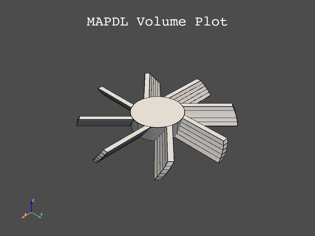
To create an image with PyMAPDL, you can add this code to the
rotor.py file:
mapdl.vplot(savefig="volumes.jpg")
To add a frame, you can use ImageMagick:
mogrify -mattecolor \#f1ce80 -frame 10x10 volumes.jpg
You can also use Imagemagick to add a watermark:
COMPOSITE=/usr/bin/composite
$COMPOSITE -gravity SouthEast watermark.jpg volumes.jpg volumes_with_watermark.jpg
Here are descriptions for values used in the preceding code:
-gravity: Location of the watermark in case the watermark is smaller than the image.COMPOSITE: Path to the ImageMagickcompositefunction.watermark.png: Name of the PNG file with the watermark image.volumes_with_watermark.jpg: Name of the JPG file to save the output to.
The final results should look like the ones in this image:
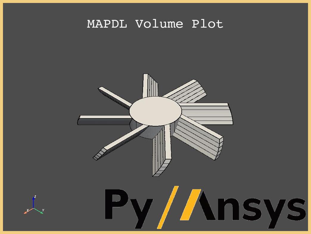
Volumes image with watermark#
Usage on the cloud#
Using these concepts, you can deploy your own apps to the cloud.
For example, you can execute the previous example on a GitHub runner using this approach (non-tested):
my_job:
   name: 'Generate watermarked images'
   runs-on: ubuntu-latest

   steps:
      - name: "Install Git and check out project"
        uses: actions/checkout@v4

      - name: "Set up Python"
        uses: actions/setup-python@v4

      - name: "Install ansys-mapdl-core"
        run: |
            python -m pip install ansys-mapdl-core

      - name: "Install ImageMagic"
        run: |
         sudo apt install imagemagick

      - name: "Generate images with PyMAPDL"
        run: |
         python rotor.py 4 --density 7000

      - name: "Postprocessing images"
        run: |
           COMPOSITE=/usr/bin/composite
           mogrify -mattecolor #f1ce80 -frame 10x10 volume.jpg
           $COMPOSITE -gravity SouthEast watermark.jpg volumes.jpg volumes_with_watermark.jpg
Additional files#
You can use these links to download the example files:
Original
rotor.pyscriptApp
cli_rotor.pyscript