Note
Go to the end to download the full example code
Structural Analysis of a Lathe Cutter#
Basic walk through PyMAPDL capabilities.
Objective#
The objective of this example is to highlight some regularly used PyMAPDL features via a lathe cutter finite element model. Lathe cutters have multiple avenues of wear and failure, and the analyses supporting their design would most often be transient thermal-structural. However, for simplicity, this simulation example uses a non-uniform load.
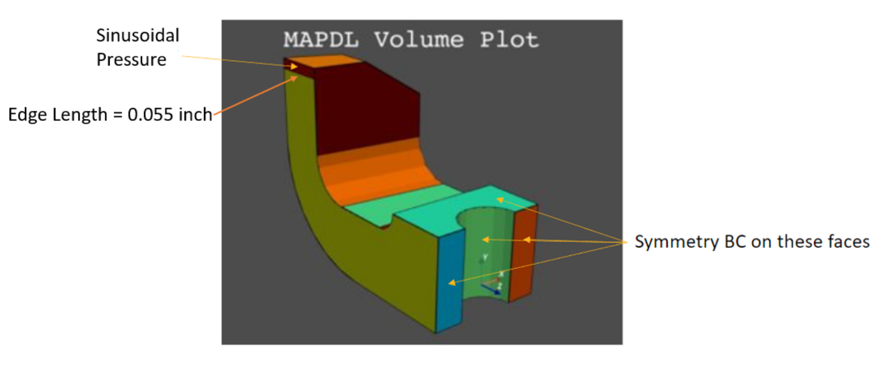
Figure 1: Lathe cutter geometry and load description.#
Contents#
Variables and launch Define necessary variables and launch MAPDL.
Geometry, mesh, and MAPDL parameters Import geometry and inspect for MAPDL parameters. Define linear elastic material model with Python variables. Mesh and apply symmetry boundary conditions.
Coordinate system and load Create a local coordinate system for the applied load and verify with a plot.
Pressure load Define the pressure load as a sine function of the length of the application area using numpy arrays. Import the pressure array into MAPDL as a table array. Verify the applied load and solve.
Plotting Show result plotting, plotting with selection, and working with the plot legend.
Postprocessing: List a result two ways: use PyMAPDL and the Pythonic version of APDL. Demonstrate extended methods and writing a list to a file.
Advanced plotting Use of
pyvista.UnstructuredGridfor additional postprocessing.
Step 1: Variables and launch#
Define variables and launch MAPDL.
Often used MAPDL command line options are exposed as Pythonic parameter names in
ansys.mapdl.core.launch_mapdl(). For example, -dir
has become run_location.
You could use run_location to specify the MAPDL run location. For example:
mapdl = launch_mapdl(run_location=path)
Otherwise, the MAPDL working directory is stored in mapdl.directory. In this
directory, MAPDL will create some of the images we will show later.
Options without a Pythonic version can be accessed by the additional_switches
parameter.
Here -smp is used only to keep the number of solver files to a minimum.
mapdl = launch_mapdl(additional_switches="-smp")
Step 2: Geometry, mesh, and MAPDL parameters#
Import geometry and inspect for MAPDL parameters.
Define material and mesh, and then create boundary conditions.
# First, reset the MAPDL database.
mapdl.clear()
Import the geometry file and list any MAPDL parameters.
lathe_cutter_geo = download_example_data("LatheCutter.anf", "geometry")
mapdl.input(lathe_cutter_geo)
mapdl.finish()
print(mapdl.parameters)
MAPDL Parameters
----------------
PRESS_LENGTH                     : 0.055
UNIT_SYSTEM                      : "bin"
Use pressure area per length in the load definition.
pressure_length = mapdl.parameters["PRESS_LENGTH"]

print(mapdl.parameters)
MAPDL Parameters
----------------
PRESS_LENGTH                     : 0.055
UNIT_SYSTEM                      : "bin"
Change the units and title.
mapdl.units("Bin")
mapdl.title("Lathe Cutter")
TITLE=
 Lathe Cutter
Set material properties.
MATERIAL 1 NUXY = 0.2700000
The MAPDL element type SOLID285 is used for demonstration purposes.
Consider using an appropriate element type or mesh density for your actual
application.
mapdl.et(1, 285)
mapdl.smrtsize(4)
mapdl.aesize(14, 0.0025)
mapdl.vmesh(1)

mapdl.da(11, "symm")
mapdl.da(16, "symm")
mapdl.da(9, "symm")
mapdl.da(10, "symm")
CONSTRAINT AT AREA    10
      LOAD LABEL = SYMM
Step 3: Coordinate system and load#
Create a local Coordinate System (CS) for the applied pressure as a function of local X.
Local CS ID is 11
mapdl.cskp(11, 0, 2, 1, 13)
mapdl.csys(1)
mapdl.view(1, -1, 1, 1)
mapdl.psymb("CS", 1)
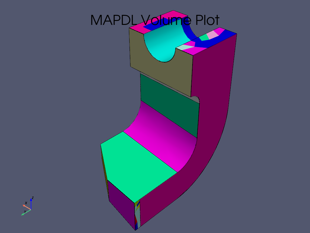
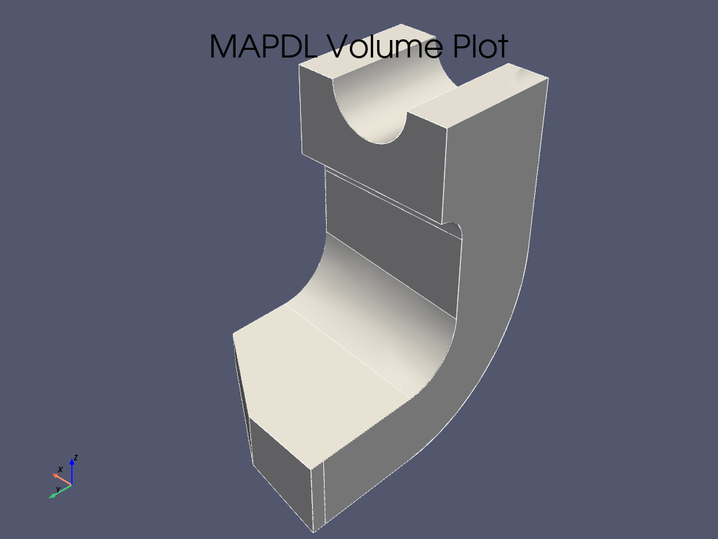
mapdl.vplot(
color_areas=True,
show_lines=True,
cpos=[-1, 1, 1],
smooth_shading=True,
)
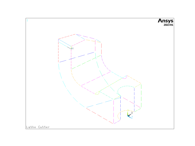
VTK plots do not show MAPDL plot symbols.
However, to use MAPDL plotting capabilities, you can set the keyword
option vtk to False.
mapdl.lplot(vtk=False)
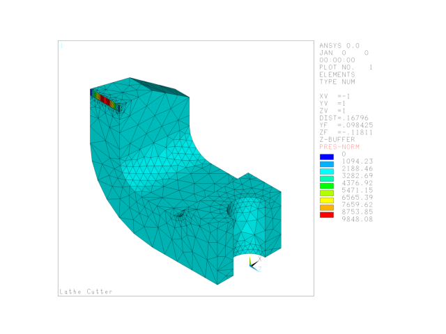
Step 4: Pressure load#
Create a pressure load, load it into MAPDL as a table array, verify the load, and solve.
length_x and press are vectors. To combine them into the correct
form needed to define the MAPDL table array, you can use
numpy.stack.
SELECT ALL ENTITIES OF TYPE= ALL AND BELOW
You can open the MAPDL GUI to check the model.
mapdl.open_gui()
Set up the solution.
mapdl.finish()
mapdl.slashsolu()
mapdl.nlgeom("On")
mapdl.psf("PRES", "NORM", 3, 0, 1)
mapdl.view(1, -1, 1, 1)
mapdl.eplot(vtk=False)
Solve the model.
mapdl.solve()
mapdl.finish()
if mapdl.solution.converged:
    print("The solution has converged.")
The solution has converged.
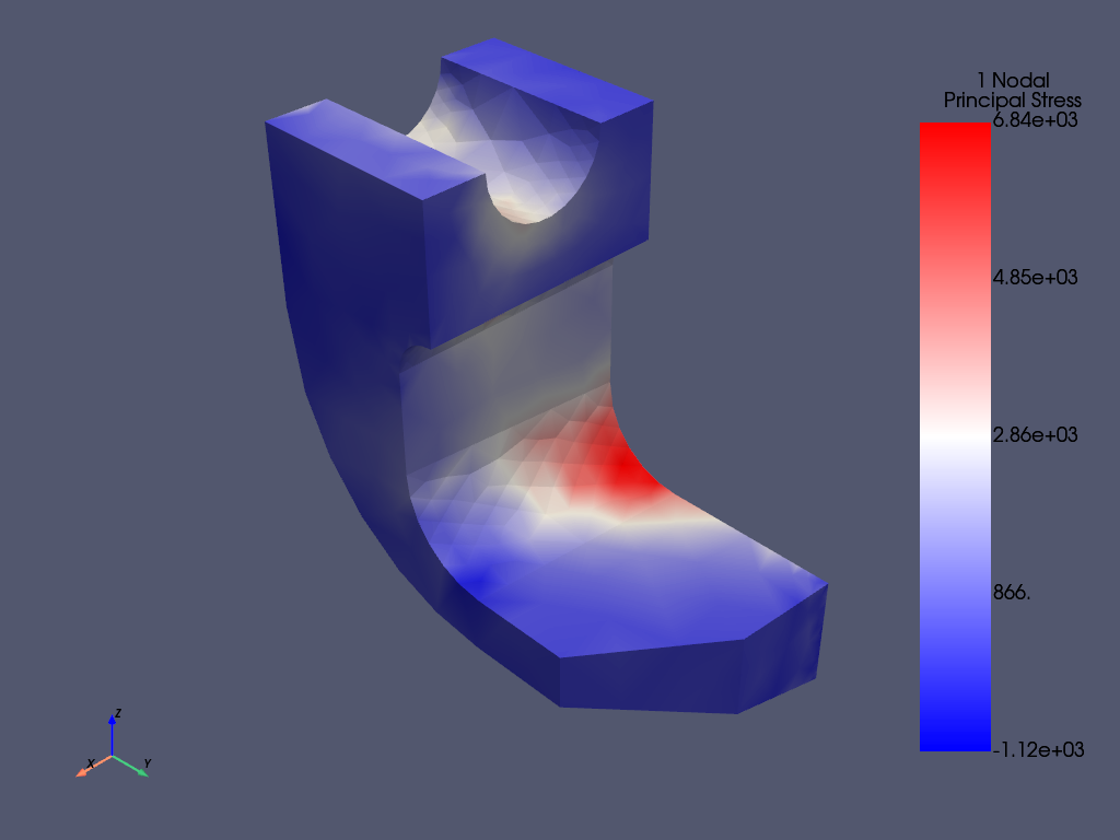
Step 5: Plotting#
mapdl.post1()
mapdl.set("last")
mapdl.allsel()

mapdl.post_processing.plot_nodal_principal_stress("1", smooth_shading=False)
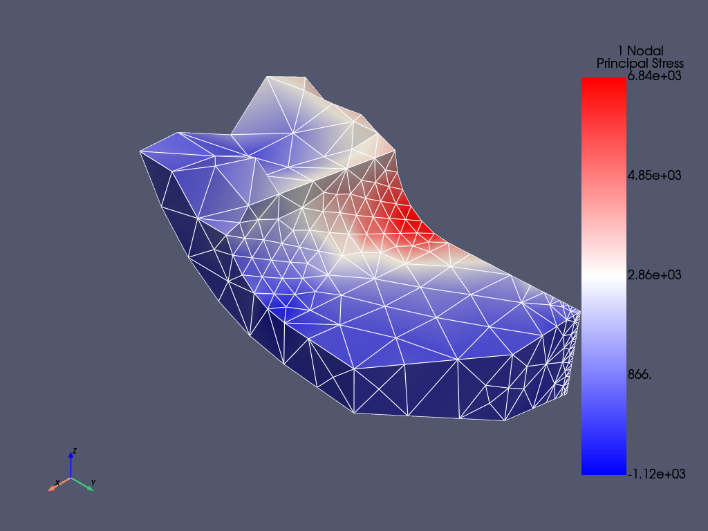
Plotting - Part of Model#
mapdl.csys(1)
mapdl.nsel("S", "LOC", "Z", -0.5, -0.141)
mapdl.esln()
mapdl.nsle()
mapdl.post_processing.plot_nodal_principal_stress(
    "1", edge_color="white", show_edges=True
)
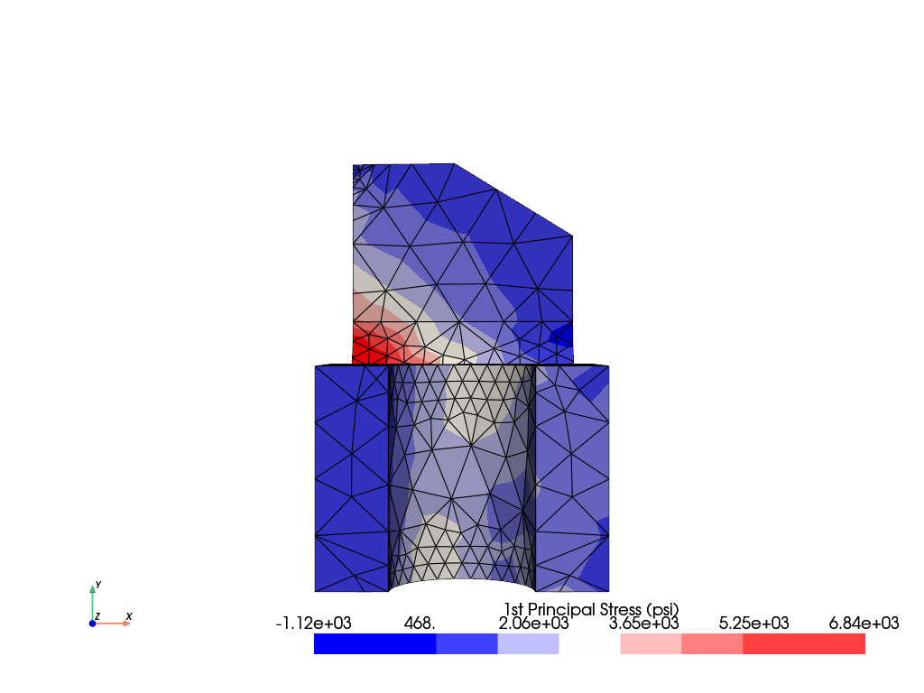
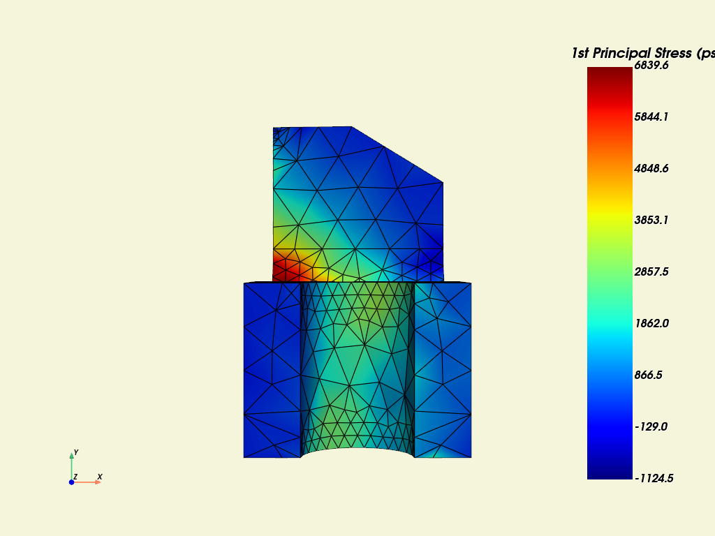
Plotting - Legend Options#
mapdl.allsel()
sbar_kwargs = {
    "color": "black",
    "title": "1st Principal Stress (psi)",
    "vertical": False,
    "n_labels": 6,
}
mapdl.post_processing.plot_nodal_principal_stress(
    "1",
    cpos="xy",
    background="white",
    edge_color="black",
    show_edges=True,
    scalar_bar_args=sbar_kwargs,
    n_colors=9,
)
Let’s try out some scalar bar options from the PyVista documentation. For example, let’s set black text on a beige background.
The scalar bar keywords defined as a Python dictionary are an alternate method to using {key:value}’s. You can use the click-and drag method to reposition the scalar bar. Left-click it and hold down the left mouse button while moving the mouse.
sbar_kwargs = dict(
    title_font_size=20,
    label_font_size=16,
    shadow=True,
    n_labels=9,
    italic=True,
    bold=True,
    fmt="%.1f",
    font_family="arial",
    title="1st Principal Stress (psi)",
    color="black",
)

mapdl.post_processing.plot_nodal_principal_stress(
    "1",
    cpos="xy",
    edge_color="black",
    background="beige",
    show_edges=True,
    scalar_bar_args=sbar_kwargs,
    n_colors=256,
    cmap="jet",
)

# cmap names *_r usually reverses values.  Try cmap='jet_r'
Step 6: Postprocessing#
Results List#
Get all principal nodal stresses.
mapdl.post_processing.nodal_principal_stress("1")
array([1198.57552642, 1308.34503077,  111.30925963, ..., 1661.40055342,
       1323.07883419, 1360.64830088])
Get the principal nodal stresses of the node subset.
mapdl.nsel("S", "S", 1, 6700, 7720)
mapdl.esln()
mapdl.nsle()

print("The node numbers are:")
print(mapdl.mesh.nnum)  # get node numbers

print("The principal nodal stresses are:")
mapdl.post_processing.nodal_principal_stress("1")
The node numbers are:
[  84   85  415  416  417  425  426 1104 1163]
The principal nodal stresses are:

array([7283.37637597, 7651.99689433, 7308.07851329, 6839.63086963,
       7173.27831228, 6892.53836453, 6399.20826385, 6607.44852844,
       5994.1721867 ])
Results as lists, arrays, and DataFrames#
Using mapdl.prnsol() to check
print(mapdl.prnsol("S", "PRIN"))
PRINT S    NODAL SOLUTION PER NODE
   *****MAPDL VERIFICATION RUN ONLY*****
     DO NOT USE RESULTS FOR PRODUCTION

  ***** POST1 NODAL STRESS LISTING *****

  LOAD STEP=     1  SUBSTEP=     1
   TIME=    1.0000      LOAD CASE=   0

    NODE     S1           S2           S3           SINT         SEQV
      84   7283.4       300.35       212.68       7070.7       7027.3
      85   7652.0       962.92       23.004       7629.0       7205.2
     415   7308.1       489.51       267.33       7040.7       6932.3
     416   6839.6       329.26       133.98       6705.7       6610.2
     417   7173.3       371.75       119.59       7053.7       6931.1
     425   6892.5       310.35      -121.13       7013.7       6808.2
     426   6399.2       283.26       12.246       6387.0       6255.9
    1104   6607.4       417.21       163.29       6444.2       6321.0
    1163   5994.2      -215.18      -712.68       6706.9       6472.5

 MINIMUM VALUES
 NODE          0            0            0            0            0
 VALUE    5994.2      -215.18      -712.68       6387.0       6255.9

 MAXIMUM VALUES
 NODE          0            0            0            0            0
 VALUE    7652.0       962.92       267.33       7629.0       7205.2
Use this command to obtain the data as a list.
mapdl_s_1_list = mapdl.prnsol("S", "PRIN").to_list()
print(mapdl_s_1_list)
[[84.0, 7283.4, 300.35, 212.68, 7070.7, 7027.3], [85.0, 7652.0, 962.92, 23.004, 7629.0, 7205.2], [415.0, 7308.1, 489.51, 267.33, 7040.7, 6932.3], [416.0, 6839.6, 329.26, 133.98, 6705.7, 6610.2], [417.0, 7173.3, 371.75, 119.59, 7053.7, 6931.1], [425.0, 6892.5, 310.35, -121.13, 7013.7, 6808.2], [426.0, 6399.2, 283.26, 12.246, 6387.0, 6255.9], [1104.0, 6607.4, 417.21, 163.29, 6444.2, 6321.0], [1163.0, 5994.2, -215.18, -712.68, 6706.9, 6472.5]]
Use this command to obtain the data as an array:
mapdl_s_1_array = mapdl.prnsol("S", "PRIN").to_array()
print(mapdl_s_1_array)
[[  84.    7283.4    300.35   212.68  7070.7   7027.3  ]
 [  85.    7652.     962.92    23.004 7629.    7205.2  ]
 [ 415.    7308.1    489.51   267.33  7040.7   6932.3  ]
 [ 416.    6839.6    329.26   133.98  6705.7   6610.2  ]
 [ 417.    7173.3    371.75   119.59  7053.7   6931.1  ]
 [ 425.    6892.5    310.35  -121.13  7013.7   6808.2  ]
 [ 426.    6399.2    283.26    12.246 6387.    6255.9  ]
 [1104.    6607.4    417.21   163.29  6444.2   6321.   ]
 [1163.    5994.2   -215.18  -712.68  6706.9   6472.5  ]]
or as a DataFrame:
mapdl_s_1_df = mapdl.prnsol("S", "PRIN").to_dataframe()
mapdl_s_1_df.head()
Use this command to obtain the data as a DataFrame, which is a. Pandas data type. Because the Pandas module is imported, you can use its functions. For example, you can write principal stresses to a file.
# mapdl_s_1_df.to_csv(path + '\prin-stresses.csv')
# mapdl_s_1_df.to_json(path + '\prin-stresses.json')
mapdl_s_1_df.to_html(path + "\prin-stresses.html")
Step 7: Advanced plotting#
mapdl.allsel()
principal_1 = mapdl.post_processing.nodal_principal_stress("1")
Load this result into the VTK grid.
grid = mapdl.mesh.grid
grid["p1"] = principal_1

sbar_kwargs = {
    "color": "black",
    "title": "1st Principal Stress (psi)",
    "vertical": False,
    "n_labels": 6,
}
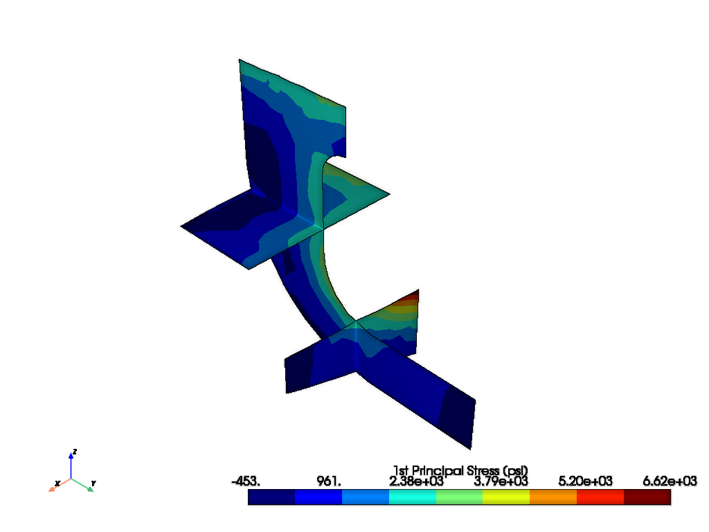
Generate a single horizontal slice along the XY plane.
Note
PyVista’s eye_dome_lighting method is used here to enhance the plots of the slices.
For more information, see`Eye Dome Lighting <pyvista_eye_dome_lighting>`_.
single_slice = grid.slice(normal=[0, 0, 1], origin=[0, 0, 0])
single_slice.plot(
    scalars="p1",
    background="white",
    lighting=False,
    eye_dome_lighting=True,
    show_edges=False,
    cmap="jet",
    n_colors=9,
    scalar_bar_args=sbar_kwargs,
)
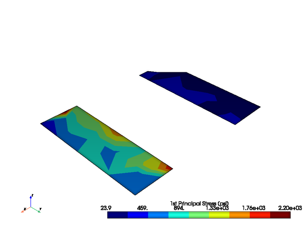
Generate a plot with three slice planes.
slices = grid.slice_orthogonal()
slices.plot(
    scalars="p1",
    background="white",
    lighting=False,
    eye_dome_lighting=True,
    show_edges=False,
    cmap="jet",
    n_colors=9,
    scalar_bar_args=sbar_kwargs,
)
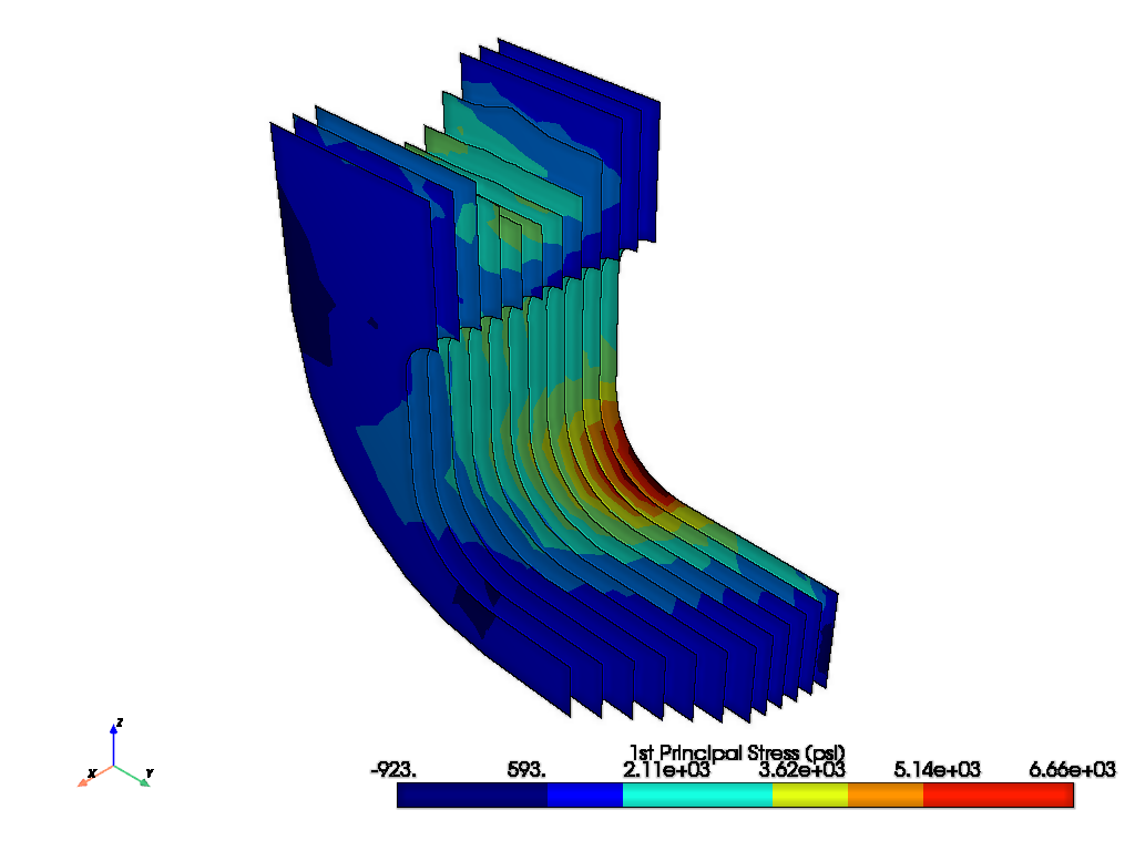
Generate a grid with multiple slices in the same plane.
slices = grid.slice_along_axis(12, "x")
slices.plot(
    scalars="p1",
    background="white",
    show_edges=False,
    lighting=False,
    eye_dome_lighting=True,
    cmap="jet",
    n_colors=9,
    scalar_bar_args=sbar_kwargs,
)
Finally, exit MAPDL.
mapdl.exit()
Total running time of the script: (0 minutes 10.615 seconds)