Stochastic finite element method with PyMAPDL#

This example leverages PyMAPDL for stochastic finite element method (SFEM) analysis using the Monte Carlo simulation. This extended example demonstrates numerous advantages and workflow possibilities that PyMAPDL provides. It explains important theoretical concepts before presenting the example.

Introduction#

Often in a mechanical system, system parameters (such as geometry, materials, and loads) and response parameters (such as displacement, strain, and stress) are taken to be deterministic. This simplification, while sufficient for a wide range of engineering applications, results in a crude approximation of actual system behavior.

To obtain a more accurate representation of a physical system, it is essential to consider the randomness in system parameters and loading conditions, along with the uncertainty in their estimation and their spatial variability. The finite element method is undoubtedly the most widely used tool for solving deterministic physical problems today. To account for randomness and uncertainty in the modeling of engineering systems, the SFEM was introduced.

SFEM extends the classical deterministic finite element approach to a stochastic framework, offering various techniques for calculating response variability. Among these, Monte Carlo simulation (MCS) stands out as the most prominent method. Renowned for its versatility and ease of implementation, MCS can be applied to virtually any type of problem in stochastic analysis.

Random variables versus stochastic processes#

This section explains how random variables and stochastic processes differ. Because these concepts are used for modeling the system randomness, explaining them is important. Random variables are easier to understand from elementary probability theory, which isn’t the case for stochastic processes. If the following explanations are too brief, consult books on SFEM. Both [1] and [2] are recommended resources.

Random variables#

Definition: A random variable is a rule for assigning to every possible outcome $θ$ of an experiment a number $X (θ)$ . For notational convenience, the dependence on $θ$ is usually dropped and the random variable is written as $X$ .

Practical example#

Imagine a beam with a concentrated load $P$ applied at a specific point. The value of $P$ is uncertain. It could vary due to manufacturing tolerances, loading conditions, or measurement errors. Here is a mathematical representation:

P : Θ ⟶ R

In the preceding equation, $Θ$ is the sample space of all possible loading scenarios, and $R$ represents the set of possible load magnitudes. For example, $P$ could be modeled as a random variable with a probability density function (PDF):

f_{P} (p) = \frac{1}{\sqrt{2 π σ^{2}}} e^{- \frac{(p - μ)^{2}}{2 σ^{2}}},

Here $μ$ is the mean load, and $σ^{2}$ is its variance.

Stochastic processes#

Definition: Recall that a random variable is defined as a rule that assigns a number $X$ to every outcome $θ$ of an experiment. However, in some applications, the experiment evolves with respect to a deterministic parameter $t$ , which belongs to an interval $I$ . For example, this occurs in an engineering system subjected to random dynamic loads over a time interval $I \subseteq R^{+}$ . In such cases, the system’s response at a specific material point is described not by a single random variable but by a collection of random variables ${X (t)}$ indexed by $t \in I$ .

This infinite collection of random variables over the interval $I$ is called a stochastic process and is denoted as ${X (t), t \in I}$ or simply $X$ . In this way, a stochastic process generalizes the concept of a random variable as it assigns to each outcome $θ$ of the experiment a function $X (t, θ)$ , known as a realization or sample function. Lastly, if $X$ is indexed by some spatial coordinate $s \in D \subseteq R^{n}$ rather than time $t$ , then ${X (s), s \in D}$ is called a random field.

Practical example#

Consider the material property of the beam, such as Young’s modulus $E (x)$ , which may vary randomly along the length of the beam $x$ . Instead of being a single random value, $E (x)$ is a random field. Its value is uncertain at each point along the domain, and it changes continuously across the beam. Mathematically, $E (x)$ is a random field:

E (x) : x \in [0, L] ⟶ R

Here:

$x$ is the spatial coordinate along the length of the beam ( $x \in [0, L]$ ).
$E (x)$ is a random variable at each point $x$ , and its randomness is described by a covariance function or an autocorrelation function.

For example, $E (x)$ could be a Gaussian random field, in which case it has the stationarity property, making its statistics completely defined by its mean ( $μ_{E}$ ), standard deviation ( $σ_{E}$ ), and covariance function $C_{E} (x_{i}, x_{j})$ . This stationarity simply means that the mean and standard deviation of every random variable $E (x)$ is constant and equal to $μ_{E}$ and $σ_{E}$ respectively. $C_{E} (x_{i}, x_{j})$ describes how random variables $E (x_{i})$ and $E (x_{j})$ are related. For a zero-mean Gaussian random field, the covariance function is given by this equation:

C_{E} (x_{i}, x_{j}) = σ_{E}^{2} e^{- \frac{| x_{i} - x_{j} |}{ℓ}}

Here $σ_{E}^{2}$ is the variance, and $ℓ$ is the correlation length parameter.

To aid understanding, the figure following diagram depicts two equivalent ways of visualizing a stochastic process or random field, that is, as an infinite collection of random variables or as a realization or sample function assigned to each outcome of an experiment.

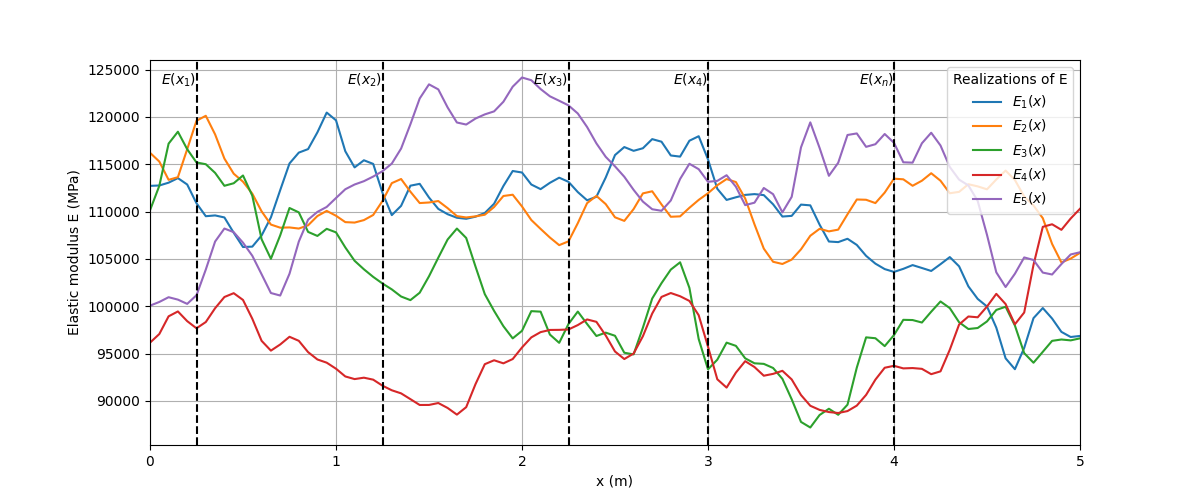
../../../_images/realizations.png — A random field $E (x)$ viewed as a collection of random variables or as realizations.#

Note

The concepts in the preceding topics generalize to more dimensions, for example, a random vector instead of a random variable, or an $R^{d}$ -valued stochastic process. A detailed discussion of these generalizations can be found in [1] and [2].

Series expansion of stochastic processes#

Since a stochastic process involves an infinite number of random variables, most engineering applications involving stochastic processes are mathematically and computationally intractable if there isn’t a way of approximating them with a series of a finite number of random variables. The next topic explains the series expansion method used in this example.

Karhunen-Loève (K-L) series expansion for a Gaussian process#

The K-L expansion of any process is based on a spectral decomposition of its covariance function. Analytical solutions are possible in a few cases, and such is the case of a Gaussian process.

For a zero-mean stationary Gaussian process, $X (t)$ , with covariance function $C_{X} (t_{i}, t_{j}) = σ_{X}^{2} e^{- \frac{| t_{i} - t_{j} |}{b}}$ defined on a symmetric domain $D = [- a, a]$ , the K-L series expansion is given by this equation:

(1)#

X (t) = \sum_{n = 1}^{\infty} \sqrt{λ_{c, n}} \cdot φ_{c, n} (t) \cdot ξ_{c, n} + \sum_{n = 1}^{\infty} \sqrt{λ_{s, n}} \cdot φ_{s, n} (t) \cdot ξ_{s, n}, t \in D

The terms in the first summation are given by

(2)#

\begin{array}{r} \begin{matrix} λ_{c, n} = \frac{2 b}{1 + ω_{c, n}^{2} \cdot b^{2}}, φ_{c, n} (t) = k_{c, n} \cos (ω_{c, n} \cdot t) \\ k_{c, n} = \frac{1}{\sqrt{a + \frac{\sin (2 ω_{c, n} \cdot a)}{2 ω_{c, n}}}} \end{matrix} \end{array}

In the preceding terms, $ω_{c, n}$ is obtained as the solution of

(3)#

\frac{1}{b} - ω_{c, n} \cdot \tan (ω_{c, n} \cdot a) = 0 in the range [(n - 1) \frac{π}{a}, (n - \frac{1}{2}) \frac{π}{a}]

The terms in the second summation are given by

(4)#

\begin{array}{r} \begin{matrix} λ_{s, n} = \frac{2 b}{1 + ω_{s, n}^{2} \cdot b^{2}}, φ_{s, n} (t) = k_{s, n} \sin (ω_{s, n} \cdot t) \\ k_{s, n} = \frac{1}{\sqrt{a - \frac{\sin (2 ω_{s, n} \cdot a)}{2 ω_{s, n}}}} \end{matrix} \end{array}

In the preceding terms, $ω_{s, n}$ is obtained as the solution of

(5)#

\frac{1}{b} \cdot \tan (ω_{s, n} \cdot a) + ω_{s, n} = 0 in the range [(n - \frac{1}{2}) \frac{π}{a}, n \frac{π}{a}]

It is worth mentioning that $λ$ and $ω$ in the series expansion are referred to as eigenvalue and frequency respectively.

Note

In the case of an asymmetric domain, such as $D = [- t_{m i n}, t_{m a x}]$ , a shift parameter $T = (t_{m i n} + t_{m a x}) / 2$ is required and the corresponding symmetric domain becomes defined by this equation:

D^{'} = D - T = [\frac{t_{m i n} - t_{m a x}}{2}, \frac{t_{m a x} - t_{m i n}}{2}]

The series expansion is then defined by this equation:

X (t) = \sum_{n = 1}^{\infty} \sqrt{λ_{c, n}} \cdot φ_{c, n} (t - T) \cdot ξ_{c, n} + \sum_{n = 1}^{\infty} \sqrt{λ_{s, n}} \cdot φ_{s, n} (t - T) \cdot ξ_{s, n}, t \in D

The K-L expansion of a Gaussian process has the property that $ξ_{c, n}$ and $ξ_{s, n}$ are independent standard normal variables, that is they follow the $N (0, 1)$ distribution. Another property is that $λ_{c, n}$ and $λ_{s, n}$ converge to zero fast (in the mean square sense). For practical implementation, this means that the infinite series of the K-L expansion is truncated after a finite number of terms, giving the approximation:

(6)#

X (t) \approx \hat{X} (t) = \sum_{n = 1}^{P} \sqrt{λ_{c, n}} \cdot φ_{c, n} (t) \cdot ξ_{c, n} + \sum_{n = 1}^{Q} \sqrt{λ_{s, n}} \cdot φ_{s, n} (t) \cdot ξ_{s, n}

Equation (6) is computationally feasible to handle. A summary of how to use it to generate realizations of $X (t)$ follows:

To generate the j-th realization, draw a random value for each $ξ_{c, n}, n = 1, \dots, P, ξ_{s, n}, n = 1, \dots, Q$ from the standard normal distribution $N (0, 1)$ and obtain $ξ_{c, 1}^{j}, \dots, ξ_{c, P}^{j}, ξ_{s, 1}^{j}, \dots, ξ_{s, P}^{j}$
Insert these values into equation (6) in other to obtain the j-th realization:

{\hat{X}}^{j} (t) = \sum_{n = 1}^{P} \sqrt{λ_{c, n}} \cdot φ_{c, n} (t) \cdot ξ_{c, n}^{j} + \sum_{n = 1}^{Q} \sqrt{λ_{s, n}} \cdot φ_{s, n} (t) \cdot ξ_{s, n}^{j}

To generate additional realizations, simply draw new random values for $ξ_{c, n}, n = 1, \dots, P, ξ_{s, n}, n = 1, \dots, Q$ each from $N (0, 1)$ .

Note

In this case of a field, the preceding discussion applies as the only difference is a change in notation (for example $t$ to $x$ ).

Monte Carlo simulation#

For linear static problems in the context of FEM, the system equations that must be solved change. The well-known deterministic equation defined by:

K K U U = F F

changes to

K K (ξ ξ) U U (ξ ξ) = F F (ξ ξ)

Here $ξ ξ$ collects sources of system randomness. The Monte Carlo simulation for solving the preceding equation consists of generating a large number of $N_{s i m}$ of samples $ξ ξ, i = 1, \dots, N_{s i m}$ from their probability distribution and for each of these samples solving the deterministic problem:

K K (ξ ξ_{(i)}) U U (ξ ξ_{(i)}) = F F (ξ ξ_{(i)})

The next step is to collect the $N_{s i m}$ response vectors $U_{i} U_{i} := U U (ξ ξ_{(i)})$ and perform a statistical postprocessing to extract useful information such as mean value, variance, histogram, and empirical PDF.

Problem description#

The following plane stress problem shows a two-dimensional cantilever structure under a point load.

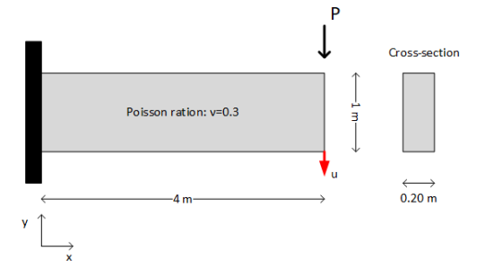
../../../_images/problem.png — A two-dimensional cantilever structure under a point load.#

$P$ is a random variable following the Gaussian distribution $N (10, 2)$ (kN), and the modulus of elasticity is a random field given by this expression:

E (x) = 10^{5} (1 + 0.10 f (x)) (k N / m^{2})

Here $f (x)$ is a zero mean stationary Gaussian field with unit variance. The covariance function for $f$ is $C_{f} (x_{r}, x_{s}) = e^{- \frac{| x_{r} - x_{s} |}{3}}$ .

Using the K-L series expansion, generate 5000 realizations for $E (x)$ and perform Monte Carlo simulation to determine the PDF of the response $u$ , at the bottom right corner of the cantilever.
If some design code stipulates that the displacement $u$ must not exceed $0.2 m$ , how confident can you be that the structure meets this requirement?

Note

This example strongly emphasizes how PyMAPDL can help to supercharge workflows. At a very high level, subsequent topics use Python libraries to handle computations related to the stochasticity of the problem and use MAPDL to run the necessary simulations all within the comfort of a Python environment.

Evaluating the Young’s modulus#

Code that allows representation of the zero-mean Gaussian field $f$ is implemented. This simply means solving the (3) and (5) and then substituting calculated values into (2) and (4) to obtain the constant terms in those equations. The number of retained terms $P$ and $Q$ in (6) can be automatically determined by structuring the code to stop computing values when $λ_{c, n}, λ_{s, n}$ become lower than a desired accuracy level. The implementation follows:

import math
import random
from typing import Callable, Tuple

import numpy as np


def find_solution(
    func: Callable[[float], float],
    derivative_func: Callable[[float], float],
    acceptable_solution_error: float,
    solution_range: Tuple[float, float],
) -> float:
    """Find the solution of g(x) = 0 within a solution range where g(x) is non-linear.

    Parameters
    ----------
    func : Callable[float, float]
        Definition of the function.
    derivative_func : Callable[float, float]
        Derivative of the preceding function.
    acceptable_solution_error : float
        Error the solution is acceptable at.
    solution_range : Tuple[float, float]
        Range for searching for the solution.

    Returns
    -------
    float
        Solution to g(x) = 0.
    """

    current_guess = random.uniform(*solution_range)
    iteration_counter = 1

    while True:
        if iteration_counter > 100:
            iteration_counter = 1
            current_guess = random.uniform(*solution_range)
            continue

        updated_guess = current_guess - func(current_guess) / derivative_func(
            current_guess
        )
        error = abs(updated_guess - current_guess)

        if error < acceptable_solution_error and not (
            solution_range[0] < updated_guess < solution_range[1]
        ):
            current_guess = random.uniform(*solution_range)
            continue
        elif error < acceptable_solution_error and (
            solution_range[0] < updated_guess < solution_range[1]
        ):
            return updated_guess

        current_guess = updated_guess
        iteration_counter += 1


def evaluate_KL_cosine_terms(
    domain: Tuple[float, float], correl_length_param: float, min_eigen_value: float
) -> Tuple[np.ndarray, np.ndarray, np.ndarray]:
    """Build array of eigenvalues and constants of the cosine terms in the KL expansion of a Gaussian stochastic process.

    Parameters
    ----------
    domain : Tuple[float, float]
        Domain for finding the KL representation of the stochastic process.
    correl_length_param : float
        Correlation length parameter of the autocorrelation function of the process.
    min_eigen_value : float
        Minimum eigenvalue to achieve required accuracy.

    Returns
    -------
    Tuple[np.ndarray, np.ndarray, np.ndarray]
        Arrays of frequencies, eigenvalues, and constants of the retained cosine terms (P in total) in the KL expansion.
    """

    A = (domain[1] - domain[0]) / 2  # Symmetric domain parameter -> [-A, A]

    frequency_array = []
    cosine_eigen_values_array = []
    cosine_constants_array = []

    # Define the functions related to the sine terms
    def func(w_n):
        return 1 / correl_length_param - w_n * math.tan(w_n * A)

    def deriv_func(w_n):
        return -w_n * A / math.cos(w_n * correl_length_param) ** 2 - math.tan(w_n * A)

    def eigen_value(w_n):
        return (2 * correl_length_param) / (1 + (correl_length_param * w_n) ** 2)

    def cosine_constant(w_n):
        return 1 / (A + (math.sin(2 * w_n * A) / (2 * w_n))) ** 0.5

    # Build the array of eigenvalues and constant terms for the accuracy required
    for n in range(1, 100):
        # start solving here
        acceptable_solution_error = 1e-10
        solution_range = [(n - 1) * math.pi / A, (n - 0.5) * math.pi / A]
        solution = find_solution(
            func, deriv_func, acceptable_solution_error, solution_range
        )

        frequency_array.append(solution)
        cosine_eigen_values_array.append(eigen_value(solution))
        cosine_constants_array.append(cosine_constant(solution))
        if eigen_value(solution) < min_eigen_value:
            break

    return (
        np.array(frequency_array),
        np.array(cosine_eigen_values_array),
        np.array(cosine_constants_array),
    )


def evaluate_KL_sine_terms(
    domain: Tuple[float, float], correl_length_param: float, min_eigen_value: float
) -> Tuple[np.ndarray, np.ndarray, np.ndarray]:
    """Build an array of eigenvalues and constants of the sine terms in the KL expansion of a gaussian stochastic process.

    Parameters
    ----------
    domain : Tuple[float, float]
        Domain for finding the KL representation of the stochastic process.
    correl_length_param : float
        Correlation length parameter of the autocorrelation function of the process.
    min_eigen_value : float
        Minimum eigenvalue to achieve required accuracy.

    Returns
    -------
    Tuple[np.ndarray, np.ndarray, np.ndarray]
        Arrays of frequencies, eigenvalues, and constants of the retained sine terms (Q in total) in the KL expansion.
    """

    A = (domain[1] - domain[0]) / 2  # Symmetric domain parameter -> [-A, A]

    frequency_array = []
    sine_eigen_values_array = []
    sine_constants_array = []

    # Define functions related to the sine terms
    def func(w_n):
        return (1 / correl_length_param) * math.tan(w_n * A) + w_n

    def deriv_func(w_n):
        return A / (correl_length_param * math.cos(w_n * A) ** 2) + 1

    def eigen_value(w_n):
        return (2 * correl_length_param) / (1 + (correl_length_param * w_n) ** 2)

    def sine_constant(w_n):
        return 1 / (A - (math.sin(2 * w_n * A) / (2 * w_n))) ** 0.5

    # Build the array of eigenvalues and constant terms for the accuracy required
    for n in range(1, 100):
        # start solving here
        acceptable_solution_error = 1e-10
        solution_range = [(n - 0.5) * math.pi / A, n * math.pi / A]
        solution = find_solution(
            func, deriv_func, acceptable_solution_error, solution_range
        )

        frequency_array.append(solution)
        sine_eigen_values_array.append(eigen_value(solution))
        sine_constants_array.append(sine_constant(solution))
        if eigen_value(solution) < min_eigen_value:
            break

    return (
        np.array(frequency_array),
        np.array(sine_eigen_values_array),
        np.array(sine_constants_array),
    )

The next step is to put this all together in a function that expresses the $f$ using the (6) equation:

def stochastic_field_realization(
    cosine_frequency_array: np.ndarray,
    cosine_eigen_values: np.ndarray,
    cosine_constants: np.ndarray,
    cosine_random_variables_set: np.ndarray,
    sine_frequency_array: np.ndarray,
    sine_eigen_values: np.ndarray,
    sine_constants: np.ndarray,
    sine_random_variables_set: np.ndarray,
    domain: Tuple[float, float],
    evaluation_point: float,
) -> float:
    """Realization of the Gaussian field f(x).

    Parameters
    ----------
    cosine_frequency_array : np.ndarray
        Array of length P, containing the frequencies associated with the retained cosine terms.
    cosine_eigen_values : np.ndarray
        Array of length P, containing the eigenvalues associated with the retained cosine terms.
    cosine_constants : np.ndarray
        Array of length P, containing constants associated with the retained cosine terms.
    cosine_random_variables_set : np.ndarray
        Array of length P, containing the random variables drawn from N(0,1) for the cosine terms.
    sine_frequency_array : np.ndarray
        Array of length Q, containing the frequencies associated with the retained sine terms.
    sine_eigen_values : np.ndarray
        Array of length Q, containing eigenvalues associated with retained sine terms.
    sine_constants : np.ndarray
         Array of length Q, containing the constants associated with the retained sine terms.
    sine_random_variables_set : np.ndarray
         Array of length P, containing the random variable drawn from N(0,1) for the sine terms.
    domain : Tuple[float, float]
        Domain for finding the KL representation of the stochastic process.
    evaluation_point : float
        Point within the domain at which the value of a realization is required.

    Returns
    -------
    float
        Value of the realization at a given point within the domain.
    """
    # Shift parameter -> Because terms are solved in a symmetric domain [-A, A]
    T = (domain[0] + domain[1]) / 2

    # Using the array operation provided by the numpy package is much simpler for expressing the stochastic process
    cosine_function_terms = (
        np.sqrt(cosine_eigen_values)
        * cosine_constants
        * np.cos((evaluation_point - T) * cosine_frequency_array)
        * cosine_random_variables_set
    )

    sine_function_terms = (
        np.sqrt(sine_eigen_values)
        * sine_constants
        * np.sin((evaluation_point - T) * sine_frequency_array)
        * sine_random_variables_set
    )

    return np.sum(cosine_function_terms) + np.sum(sine_function_terms)

The function for evaluating the Young’s modulus itself is straight forward:

def young_modulus_realization(
    cosine_frequency_list,
    cosine_eigen_values,
    cosine_constants,
    cosine_random_variables_set,
    sine_frequency_list,
    sine_eigen_values,
    sine_constants,
    sine_random_variables_set,
    domain,
    evaluation_point,
):
    return 1e5 * (
        1
        + 0.1
        * stochastic_field_realization(
            cosine_frequency_list,
            cosine_eigen_values,
            cosine_constants,
            cosine_random_variables_set,
            sine_frequency_list,
            sine_eigen_values,
            sine_constants,
            sine_random_variables_set,
            domain,
            evaluation_point,
        )
    )

Realizations of the Young’s modulus#

You can now generate sample realizations of the Young’s modulus to see what they look like:

# Generate K-L expansion parameters
import matplotlib.pyplot as plt

domain = (0, 4)
correl_length_param = 3
min_eigen_value = 0.001

cosine_frequency_array, cosine_eigen_values, cosine_constants = (
    evaluate_KL_cosine_terms(domain, correl_length_param, min_eigen_value)
)
sine_frequency_array, sine_eigen_values, sine_constants = evaluate_KL_sine_terms(
    domain, correl_length_param, min_eigen_value
)

# See what the realizations looks like
no_of_realizations = 10
x = np.linspace(domain[0], domain[1], 101)

fig, ax = plt.subplots()
ax.set_xlabel(r"$x \: (m)$")
ax.set_ylabel(r"Realizations of $E$")
ax.grid(True)
fig.set_size_inches(15, 8)
ax.set_xlim(domain[0], domain[1])

for i in range(no_of_realizations):
    cosine_random_variables_set = np.random.normal(
        0, 1, size=len(cosine_frequency_array)
    )
    sine_random_variables_set = np.random.normal(0, 1, size=len(sine_frequency_array))

    realization = np.array(
        [
            young_modulus_realization(
                cosine_frequency_array,
                cosine_eigen_values,
                cosine_constants,
                cosine_random_variables_set,
                sine_frequency_array,
                sine_eigen_values,
                sine_constants,
                sine_random_variables_set,
                domain,
                evaluation_point,
            )
            for evaluation_point in x
        ]
    )
    ax.plot(x, realization)

plt.show()

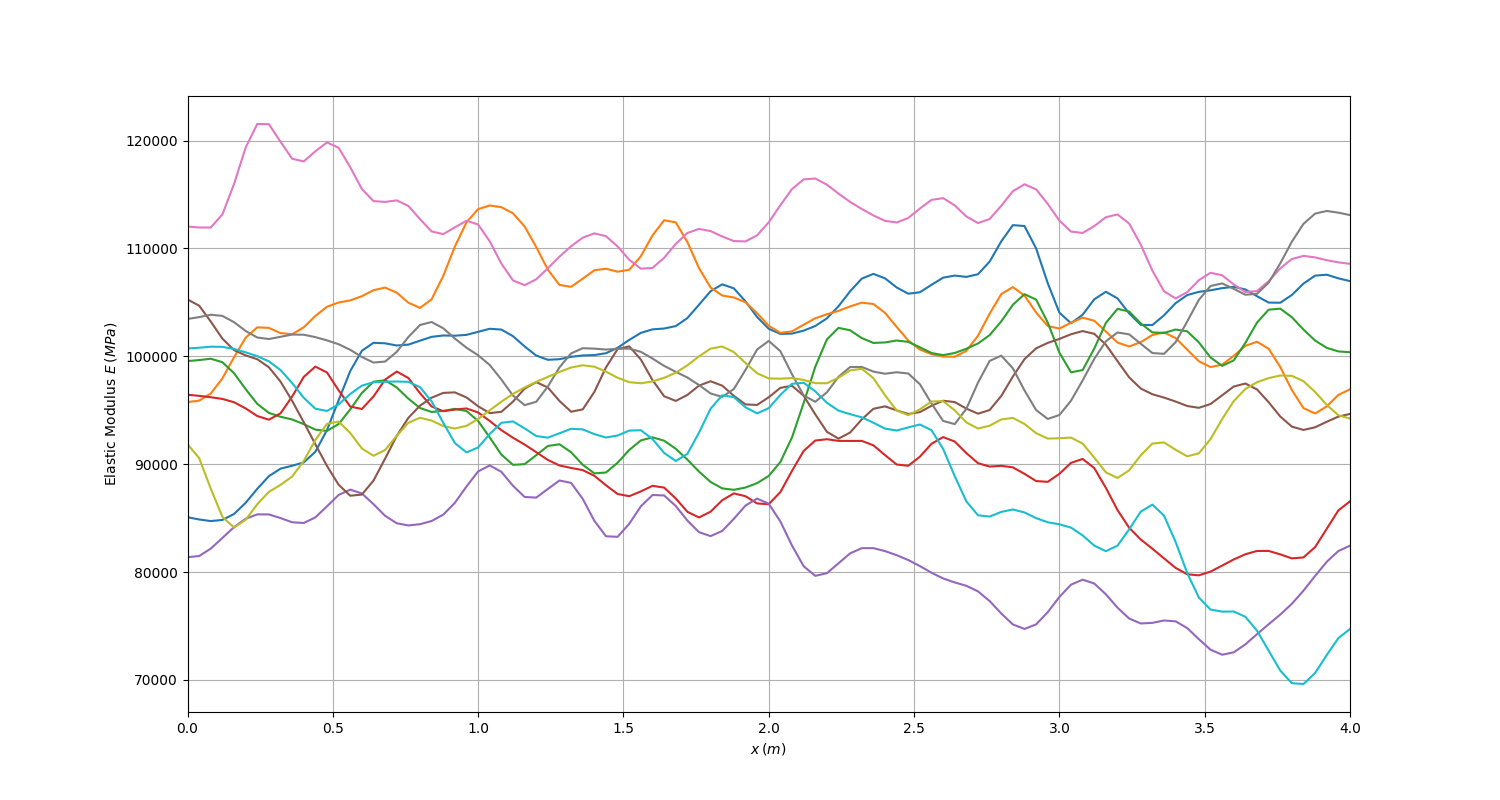
../../../_images/young_modulus_realizations.png — 10 realizations of the Young’s modulus depict randomness from one realization to another.#

Verification of the implementation#

You can compute the theoretical mean and variance of the Young’s modulus and then use them to verify the correctness of the implemented code.

For the mean:

(7)#

\begin{array}{r} \begin{matrix} E (E) = E (10^{5} (1 + 0.10 f)) \\ E (E) = 10^{5} (1 + 0.1 E (f)) \\ E (E) = 10^{5} (1 + 0.1 (0)) = 10^{5} k N / m^{2} \end{matrix} \end{array}

For the variance:

(8)#

\begin{array}{r} \begin{matrix} V a r (E) = E (E^{2}) - [E (E)]^{2} \\ V a r (E) = E [10^{10} (1 + 0.2 f + 0.01 f^{2})] - 10^{10} \\ V a r (E) = 10^{10} [1 + 0.2 E (f) + 0.01 E (f^{2})] - 10^{10} \\ V a r (E) = 10^{10} [0.2 (0) + 0.01 (1)] \\ V a r (E) = 10^{8} {k N}^{2} / m^{4} \end{matrix} \end{array}

It is expected that as the number of realizations increase indefinitely, the ensemble mean and variance should converge towards theoretical values calculated in (7) and (8).

Firstly, several realizations are generated. 5000 is enough, which is the same as the number of simulations to be run later on. Statistical processing is then performed on these realizations.

# Verify that the previous implementation represents the Young's modulus
no_of_realizations = 5000
x = np.linspace(domain[0], domain[1], 101)
realization_collection = np.zeros((no_of_realizations, len(x)))

for i in range(no_of_realizations):
    cosine_random_variables_set = np.random.normal(
        0, 1, size=len(cosine_frequency_array)
    )
    sine_random_variables_set = np.random.normal(0, 1, size=len(sine_frequency_array))

    realization = np.array(
        [
            young_modulus_realization(
                cosine_frequency_array,
                cosine_eigen_values,
                cosine_constants,
                cosine_random_variables_set,
                sine_frequency_array,
                sine_eigen_values,
                sine_constants,
                sine_random_variables_set,
                domain,
                evaluation_point,
            )
            for evaluation_point in x
        ]
    )

    realization_collection[i:] = realization

ensemble_mean_with_realization = np.zeros(realization_collection.shape[0])
ensemble_var_with_realization = np.zeros(realization_collection.shape[0])
for i in range(realization_collection.shape[0]):
    ensemble_mean_with_realization[i] = np.mean(realization_collection[: i + 1, :])
    ensemble_var_with_realization[i] = np.var(realization_collection[: i + 1, :])

You can generate a plot of the mean versus the number of realizations:

# Plot the ensemble mean
fig, ax = plt.subplots()
fig.set_size_inches(15, 8)
ax.plot(ensemble_mean_with_realization, label="Computed mean")
ax.axhline(y=1e5, color="r", linestyle="dashed", label="Actual mean")
plt.xlabel("No of realizations")
plt.ylabel(r"Ensemble mean of $E$")
ax.grid(True)
ax.set_xlim(0, no_of_realizations)
ax.legend()
plt.show()

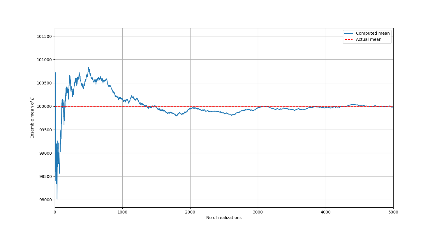
../../../_images/mean.png — The mean converges to the true value as the number of realizations is increased.#

You can also generate a plot of the variance versus the number of realizations:

# Plot of ensemble variance
fig, ax = plt.subplots()
fig.set_size_inches(15, 8)
ax.plot(ensemble_var_with_realization, label="Computed variance")
ax.axhline(y=1e8, color="r", linestyle="dashed", label="Actual variance")
plt.xlabel("No of realizations")
plt.ylabel(r"Ensemble varianc of $E$")
ax.grid(True)
ax.set_xlim(0, no_of_realizations)
ax.legend()
plt.show()

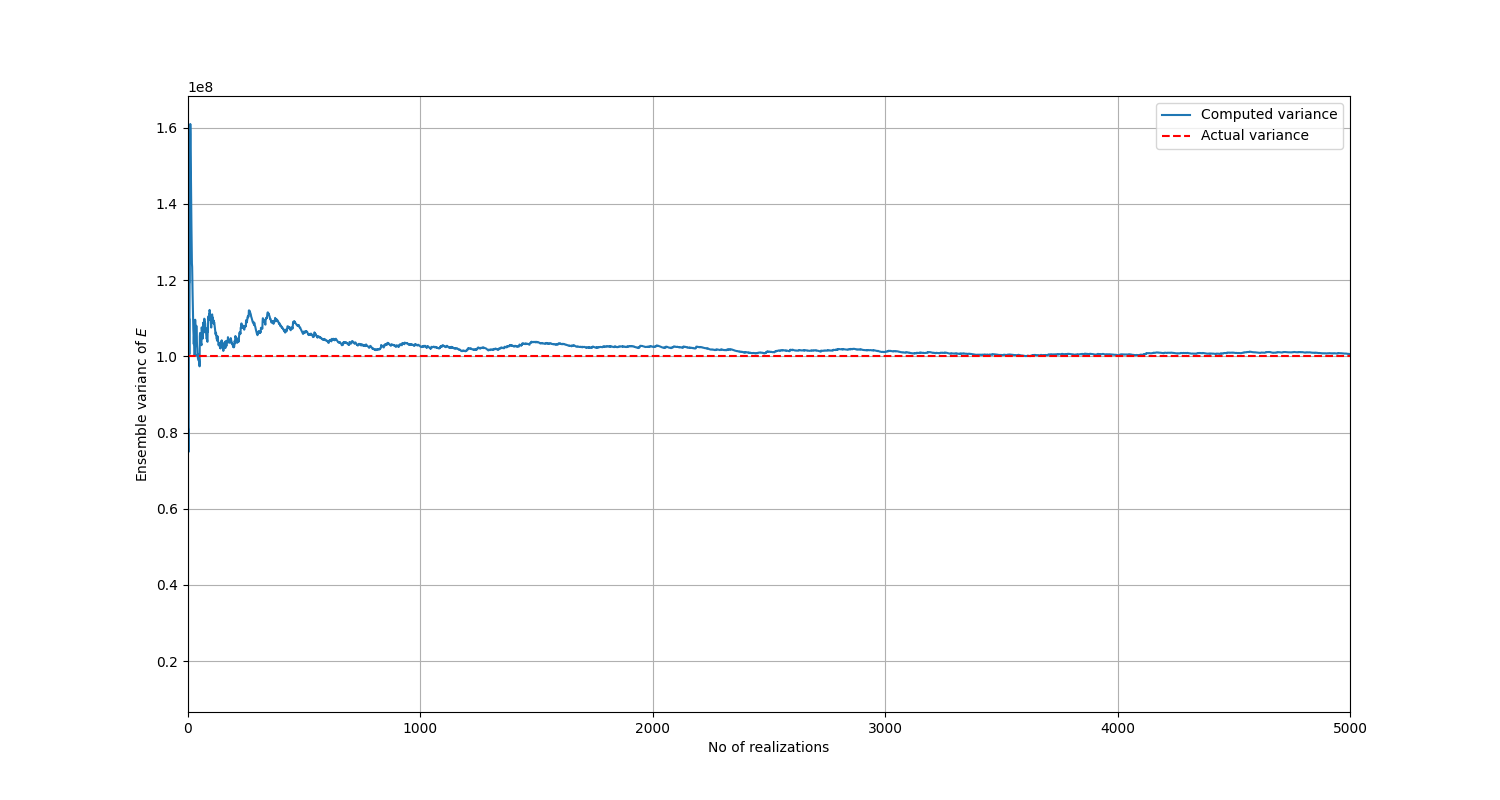
../../../_images/variance.png — The variance converges to the true value as the number of realizations is increased.#

The preceding plots confirm that the implementation is correct. If you desire more accuracy, you can further decrease the minimum eigenvalue, but the value already chosen is sufficient.

Running the simulations#

Focus now shifts to the PyMAPDL part of this example. Remember that the problem requires running 5000 simulations. Therefore, you must write a workflow that performs these actions:

Create the geometry of the cantilever model.
Mesh the model. The following code uses the four-node PLANE182 elements.
For each simulation, generate one realization of $E$ and one sample of $P$ .
For each simulation, loop through the elements and for each element, use the generated realization to assign the value of the Young’s modulus. Also assign the load for each simulation.
Solve the model and store $u$ for each simulation.

Note

One realization continuously varies with $x$ , but a plane stress element like PLANE182 can only have a constant Young’s modulus assigned. Therefore, for an element whose $x$ -coordinates are between $x_{1}$ and $x_{2}$ , you can simply assign the average value of $E$ between these two values or assign the value of $E$ at the centroid. The later is chosen for this implementation. The method chosen becomes insignificant with a finer mesh as both methods should produce similar results.

This function implements the preceding steps:

# Single-threaded approach
# Function for running the simulations
def run_simulations(
    length: float,
    height: float,
    thickness: float,
    mesh_size: float,
    no_of_simulations: int,
) -> np.ndarray:
    """Run desired number of simulations to obtain response data.

    Parameters
    ----------
    length : float
        Length of the cantilever structure.
    height : float
        Height of the cantilever structure.
    thickness : float
        Thickness of the cantilever structure.
    mesh_size : float
        Desired mesh size.
    no_of_simulations : int
       Number of simulations to run.

    Returns
    -------
    np.ndarray
        Array containing simulation results.
    """

    from pathlib import Path

    from ansys.mapdl.core import launch_mapdl

    path = Path.cwd()
    mapdl = launch_mapdl(run_location=path)

    domain = [0, length]
    correl_length_param = 3
    min_eigen_value = 0.001
    poisson_ratio = 0.3

    mapdl.prep7()  # Enter preprocessor

    mapdl.r(r1=thickness)
    mapdl.et(1, "PLANE182", kop3=3, kop6=0)
    mapdl.rectng(0, length, 0, height)
    mapdl.mshkey(1)
    mapdl.mshape(0, "2D")
    mapdl.esize(mesh_size)
    mapdl.amesh("ALL")

    # Fixed edge
    mapdl.nsel("S", "LOC", "X", 0)
    mapdl.cm("FIXED_END", "NODE")

    # Load application node
    mapdl.nsel("S", "LOC", "X", length)
    mapdl.nsel("R", "LOC", "Y", height)
    mapdl.cm("LOAD_APPLICATION_POINT", "NODE")

    mapdl.finish()  # Exit preprocessor

    mapdl.slashsolu()  # Enter solution processor

    element_ids = mapdl.esel(
        "S", "CENT", "Y", 0, mesh_size
    )  # Select bottom row elements and store the ids

    # Generate quantities required to define the Young's modulus stochastic process
    cosine_frequency_list, cosine_eigen_values, cosine_constants = (
        evaluate_KL_cosine_terms(domain, correl_length_param, min_eigen_value)
    )
    sine_frequency_list, sine_eigen_values, sine_constants = evaluate_KL_sine_terms(
        domain, correl_length_param, min_eigen_value
    )

    simulation_results = np.zeros(no_of_simulations)

    for simulation in range(no_of_simulations):
        # Generate random variables and load needed for one realization of the process
        cosine_random_variables_set = np.random.normal(
            0, 1, size=len(cosine_frequency_list)
        )
        sine_random_variables_set = np.random.normal(
            0, 1, size=len(sine_frequency_list)
        )
        load = -np.random.normal(10, 2**0.5)  # Generate a random load

        material_property = 0  # Initialize material property ID
        for element_id in element_ids:
            material_property += 1
            mapdl.get("ELEMENT_ID", "ELEM", element_id, "CENT", "X")
            element_centroid_x_coord = mapdl.parameters["ELEMENT_ID"]
            mapdl.esel(
                "S", "CENT", "X", element_centroid_x_coord
            )  # Select all elements having this coordinate as centroid

            # Evaluate Young's modulus at this material point
            young_modulus_value = young_modulus_realization(
                cosine_frequency_list,
                cosine_eigen_values,
                cosine_constants,
                cosine_random_variables_set,
                sine_frequency_list,
                sine_eigen_values,
                sine_constants,
                sine_random_variables_set,
                domain,
                element_centroid_x_coord,
            )

            mapdl.mp(
                "EX", f"{material_property}", young_modulus_value
            )  # Define property ID and assign Young's modulus
            mapdl.mp(
                "NUXY", f"{material_property}", poisson_ratio
            )  # Assign poisson ratio
            mapdl.mpchg(
                material_property, "ALL"
            )  # Assign property to selected elements

        mapdl.allsel()

        mapdl.d("FIXED_END", lab="UX", value=0, lab2="UY")  # Apply fixed end BC
        mapdl.f("LOAD_APPLICATION_POINT", lab="FY", value=load)  # Apply load BC
        mapdl.solve()

        # Displacement probe point - where Uy results are to be extracted
        displacement_probe_point = mapdl.queries.node(length, 0, 0)
        displacement = mapdl.get_value("NODE", displacement_probe_point, "U", "Y")

        simulation_results[simulation] = displacement

        mapdl.mpdele("ALL", "ALL")
        if (simulation + 1) % 10 == 0:
            print(f"Completed {simulation + 1} simulations.")

    mapdl.exit()
    print()
    print("All simulations completed.")

    return simulation_results

You can pass the required arguments to the defined function to run the simulations:

# Run the simulations
import time

start = time.time()
simulation_results = run_simulations(4, 1, 0.2, 0.1, 5000)
end = time.time()
print(
    "Simulation took {} min {} s".format(
        int((end - start) // 60), int((end - start) % 60)
    )
)

Answering problem questions#

To determine the PDF of the response $u$ , you can perform a statistical postprocessing of simulation results:

# Perform statistical postprocessing and plot the PDF
import scipy.stats as stats

kde = stats.gaussian_kde(simulation_results)  # Kernel density estimate

fig, ax = plt.subplots()
fig.set_size_inches(15, 8)
x_eval = np.linspace(min(simulation_results), max(simulation_results), num=200)
ax.plot(x_eval, kde.pdf(x_eval), "r-", label="PDF of response $u$")
plt.xlabel("Displacement in (m)")
ax.legend()
plt.show()

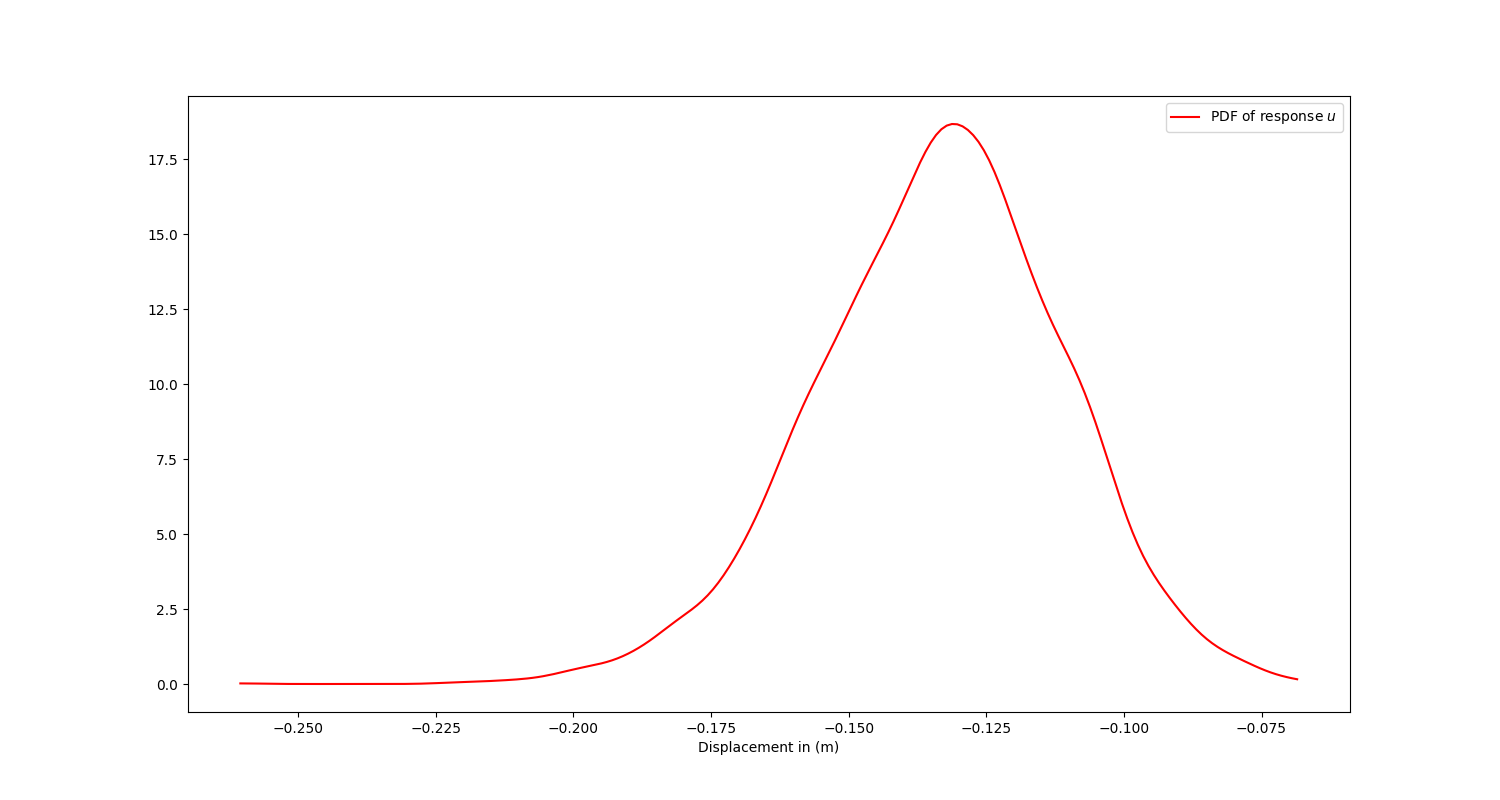
../../../_images/pdf.png — The PDF of response $u$ .#

To determine whether the structure meets the requirement of the design code, simply evaluate the probability that the response $u$ is less than $0.2 m$ :

# Proceed to evaluate the probability that the response u is less than 0.2 m
probability = kde.integrate_box_1d(-0.2, x_eval[-1])
print(f"The probability that u is less than 0.2 m is {probability:.0%}.")

The computed probability is approximately 99%, which is a measure of how well the structure satisfies the design requirement.

Note

Splitting the overall implementation of this example into several functions lets you modify practically any aspect of the problem statement with minimal edits to the code for testing out other scenarios. For example, you can use a different structural geometry, mesh size, or loading condition.

Improve simulation speed using multi-threading#

One of the main drawbacks of MCS is the number of simulations required. In this example, 5000 simulations can take quite some time to run on a single MAPDL instance. To speed things up, you can use the MapdlPool class to run simulations across multiple MAPDL instances:

# Multi-threaded approach
# Note that the number of instances should not be more than the number of available CPU cores on your PC
def run_simulations_threaded(
    mapdl, length, height, thickness, mesh_size, no_of_simulations, instance_identifier
):
    domain = [0, length]
    correl_length_param = 3
    min_eigen_value = 0.001
    poisson_ratio = 0.3

    mapdl.prep7()  # Enter preprocessor

    mapdl.r(r1=thickness)
    mapdl.et(1, "PLANE182", kop3=3, kop6=0)
    mapdl.rectng(0, length, 0, height)
    mapdl.mshkey(1)
    mapdl.mshape(0, "2D")
    mapdl.esize(mesh_size)
    mapdl.amesh("ALL")

    # Defined fixed edge
    mapdl.nsel("S", "LOC", "X", 0)
    mapdl.cm("FIXED_END", "NODE")

    # Load application node
    mapdl.nsel("S", "LOC", "X", length)
    mapdl.nsel("R", "LOC", "Y", height)
    mapdl.cm("LOAD_APPLICATION_POINT", "NODE")

    mapdl.finish()  # Exit preprocessor

    mapdl.slashsolu()  # Enter solution processor

    element_ids = mapdl.esel(
        "S", "CENT", "Y", 0, mesh_size
    )  # Select bottom row elements and store the IDs

    # Generate quantities required to define the Young's modulus stochastic process
    cosine_frequency_list, cosine_eigen_values, cosine_constants = (
        evaluate_KL_cosine_terms(domain, correl_length_param, min_eigen_value)
    )
    sine_frequency_list, sine_eigen_values, sine_constants = evaluate_KL_sine_terms(
        domain, correl_length_param, min_eigen_value
    )

    simulation_results = np.zeros(no_of_simulations)

    for simulation in range(no_of_simulations):
        # Generate random variables and the load needed for one realization of the process
        cosine_random_variables_set = np.random.normal(
            0, 1, size=len(cosine_frequency_list)
        )
        sine_random_variables_set = np.random.normal(
            0, 1, size=len(sine_frequency_list)
        )
        load = -np.random.normal(10, 2**0.5)  # Generate a random load

        material_property = 0  # Initialize material property ID
        for element_id in element_ids:
            material_property += 1
            mapdl.get("ELEMENT_ID", "ELEM", element_id, "CENT", "X")
            element_centroid_x_coord = mapdl.parameters["ELEMENT_ID"]
            mapdl.esel(
                "S", "CENT", "X", element_centroid_x_coord
            )  # Select all elements having this coordinate as centroid

            # Evaluate Young's modulus at this material point
            young_modulus_value = young_modulus_realization(
                cosine_frequency_list,
                cosine_eigen_values,
                cosine_constants,
                cosine_random_variables_set,
                sine_frequency_list,
                sine_eigen_values,
                sine_constants,
                sine_random_variables_set,
                domain,
                element_centroid_x_coord,
            )

            mapdl.mp(
                "EX", f"{material_property}", young_modulus_value
            )  # Define property ID and assign Young's modulus
            mapdl.mp(
                "NUXY", f"{material_property}", poisson_ratio
            )  # Assign Poisson ratio
            mapdl.mpchg(
                material_property, "ALL"
            )  # Assign property to selected elements

        mapdl.allsel()

        mapdl.d("FIXED_END", lab="UX", value=0, lab2="UY")  # Apply fixed end BC
        mapdl.f("LOAD_APPLICATION_POINT", lab="FY", value=load)  # Apply load BC
        mapdl.solve()

        # Displacement probe point - where Uy results are to be extracted
        displacement_probe_point = mapdl.queries.node(length, 0, 0)
        displacement = mapdl.get_value("NODE", displacement_probe_point, "U", "Y")

        simulation_results[simulation] = displacement

        mapdl.mpdele("ALL", "ALL")
        if (simulation + 1) % 10 == 0:
            print(
                f"Completed {simulation + 1} simulations in instance {instance_identifier}."
            )

    mapdl.exit()
    print()
    print(f"All simulations completed in instance {instance_identifier}.")

    return instance_identifier, no_of_simulations, simulation_results


def run_simulations_over_multple_instances(
    length, height, thickness, mesh_size, no_of_simulations, no_of_instances
):
    from pathlib import Path

    from ansys.mapdl.core import MapdlPool

    # Determine the number of simulations to run per instance
    if no_of_simulations % no_of_instances == 0:
        # Simulations can be split equally across instances
        simulations_per_instance = no_of_simulations // no_of_instances
        simulations_per_instance_list = [
            simulations_per_instance for i in range(no_of_instances)
        ]
    else:
        # Simulations cannot be split equally across instances
        simulations_per_instance = no_of_simulations // no_of_instances
        simulations_per_instance_list = [
            simulations_per_instance for i in range(no_of_instances - 1)
        ]
        remaining_simulations = no_of_simulations - sum(simulations_per_instance_list)
        simulations_per_instance_list.append(remaining_simulations)

    path = Path.cwd()
    pool = MapdlPool(no_of_instances, nproc=1, run_location=path, start_timeout=120)

    inputs = [
        (length, height, thickness, mesh_size, simulations, id + 1)
        for id, simulations in enumerate(simulations_per_instance_list)
    ]

    overall_simulation_results = pool.map(run_simulations_threaded, inputs)
    pool.exit()

    return overall_simulation_results

To run simulations over 10 MAPDL instances, call the preceding function with appropriate arguments:

# Run the simulations over several instances
start = time.time()
simulation_results = run_simulations_over_multple_instances(4, 1, 0.2, 0.1, 5000, 10)
end = time.time()
print(
    "Simulation took {} min {} s".format(
        int((end - start) // 60), int((end - start) % 60)
    )
)

# Collect the results from each instance
combined_results = [result[2] for result in simulation_results]
combined_results = np.concatenate(combined_results)

# Calculate the probability
kde = stats.gaussian_kde(combined_results)  # Kernel density estimate
probability = kde.integrate_box_1d(-0.2, max(combined_results))
print(f"The probability that u is less than 0.2 m is {probability:.0%}")

The simulations are completed much faster.

Tip

In a local test, using the MapdlPool approach (with 10 MAPDL instances) takes about 38 minutes to run, while a single instance runs for about 3 hours. The simulation speed depends on a multitude of factors, but this comparison provides an idea of the speed gain to expect when using multiple instances.

Warning

Ensure there are enough licenses available to run multiple MAPDL instances concurrently.

Stochastic finite element method with PyMAPDL#

Introduction#

Random variables versus stochastic processes#

Random variables#

Practical example#

Stochastic processes#

Practical example#

Series expansion of stochastic processes#

Karhunen-Loève (K-L) series expansion for a Gaussian process#

Monte Carlo simulation#

Problem description#

Evaluating the Young’s modulus#

Realizations of the Young’s modulus#

Verification of the implementation#

Running the simulations#

Answering problem questions#

Improve simulation speed using multi-threading#

References#