Genetic algorithms and PyMAPDL#

This example shows how to use PyMAPDL in an HPC cluster to take advantage of multiple MAPDL instances to calculate each of the genetic algorithm population solutions. To manage multiple MAPDL instances, you should use the MapdlPool class, which allows you to run multiple jobs in the background.

Introduction#

Genetic algorithms are optimization techniques inspired by the principles of natural selection and genetics. They are used to find solutions to complex problems by mimicking the process of natural selection to evolve potential solutions over successive generations. In a genetic algorithm, a population of candidate solutions (chromosomes) undergoes a series of operations, including selection, crossover, and mutation, to produce new generations of solutions. The fittest chromosomes, which best satisfy the problem constraints and objectives, are more likely to be selected for reproduction, thus gradually improving the overall quality of solutions over time. Genetic algorithms are particularly useful for solving problems where traditional methods are impractical or inefficient, such as optimization, search, and machine learning tasks. They find applications in various fields, including engineering, economics, biology, and computer science.

Problem definition#

This example shows how to use a generic algorithm to calculate the force required for a double-clamped beam to deform a specific amount in its center.

The beam model is the same as MAPDL 2D Beam Example. It is made of BEAM188 elements that span for 2.2 meters, and it fully clamped at both ends.

The PyMAPDL beam model is defined in the calculate_beam() function as follows:

def calculate_beam(mapdl, force):
    # Initialize
    mapdl.clear()
    mapdl.prep7()

    # Define an I-beam
    mapdl.et(1, "BEAM188")
    mapdl.keyopt(1, 4, 1)  # transverse shear stress output

    # Material properties
    mapdl.mp("EX", 1, 2e7)  # N/cm2
    mapdl.mp("PRXY", 1, 0.27)  # Poisson's ratio

    # Beam properties in centimeters
    sec_num = 1
    mapdl.sectype(sec_num, "BEAM", "I", "ISection", 3)
    mapdl.secoffset("CENT")
    mapdl.secdata(15, 15, 29, 2, 2, 1)  # dimensions are in centimeters

    # Set FEM model
    mapdl.n(1, 0, 0, 0)
    mapdl.n(12, 110, 0, 0)
    mapdl.n(23, 220, 0, 0)
    mapdl.fill(1, 12, 10)
    mapdl.fill(12, 23, 10)

    for node in mapdl.mesh.nnum[:-1]:
        mapdl.e(node, node + 1)

    # Define the boundary conditions
    # Allow movement only in the X and Z direction
    for const in ["UX", "UY", "ROTX", "ROTZ"]:
        mapdl.d("all", const)

    # Constrain only nodes 1 and 23 in the Z direction
    mapdl.d(1, "UZ")
    mapdl.d(23, "UZ")

    # Apply a -Z force at node 12
    mapdl.f(12, "FZ", force[0])

    # Run the static analysis
    mapdl.run("/solu")
    mapdl.antype("static")
    mapdl.solve()

    # Extract data
    UZ = mapdl.post_processing.nodal_displacement("Z")
    UZ_node_12 = UZ[12]

    return UZ_node_12

This function returns the control parameter for the model, which is the displacement at the Z-direction on the node 12 (UZ_node_12).

MAPDL pool setup#

Genetic algorithms are expensive in regard to the amount of calculations needed to reach an optimal solution. As shown earlier, many simulations must be performed to select, cross over, and mutate all the chromosomes across all the populations. For this reason, to speed up the process, it is desirable to have as many MAPDL instances as possible so that each one can calculate one chromosome fit function.

To manage multiple MAPDL instances, the best approach is to use the MapdlPool class.

# Importing packages
from ansys.mapdl.core import MapdlPool

# Start pool
# Number of instances should be equal to number of CPUs
# as set later in the ``sbatch`` command
pool = MapdlPool(n_instances=10)
print(pool)

Deflection target#

Because this is a demonstration example, the target displacement is calculated using the beam function itself with a force of 22840 $N/cm^2$.

## Define deflection target
mapdl = pool[0]  # Getting the first MAPDL instance in the pool
force = 22840  # N/cm2
target_displacement = calculate_beam(pool[0], [force])
print(f"Setting target to {target_displacement} for force {force}")

Genetic algorithm model#

Introduction#

You use the PyGAD library to configure the genetic algorithm.

PyGAD is an open source Python library for building the genetic algorithm and optimizing machine learning algorithms.

PyGAD supports different types of crossover, mutation, and parent selection operators. PyGAD allows different types of problems to be optimized using the genetic algorithm by customizing the fitness function. It works with both single-objective and multi-objective optimization problems.

From PyGAD - Python Genetic Algorithm - https://pygad.readthedocs.io/en/latest/

Configuration#

To configure the genetic algorithm, the following code is used:

# Set GA model
sol_per_pop = 20
num_generations = 10
num_parents_mating = 20
num_genes = 1  # equal to the size of inputs/outputs.
parallel_processing = ["thread", len(pool)]  # Number of parallel workers

# Initial guess limits
init_range_low = 10000
init_range_high = 30000
gene_type = int  # limit to ints

# Extra configuration
# https://blog.derlin.ch/genetic-algorithms-with-pygad
parent_selection_type = "rws"
keep_parents = 0  # No keeping parents.
mutation_percent_genes = 30
mutation_probability = 0.5

In the preceding code, the most import parameters are:

sol_per_pop: Number of solutions (chromosomes) within the population.
num_generations: Number of genes in the solution/chromosome. In this case, because only one parameter is simulated (deflection Z at node 12), this value is 1.
num_parents_mating: Number of solutions to select as parents.
parent_selection_type: Parent selection type. This example uses the rws type (for roulette wheel selection). For more information on parent selection type, see Genetic algorithms with PyGAD: selection, crossover, mutation by Lucy Linder.
parallel_processing: Number of parallel workers for the genetic algorithm and how these workers are created. They can be created as a "thread" or "process". The example creates the workers as threads, and the amount is equal to the number of instances.

Helper functions#

Additionally, for printing purposes, several helper functions are defined:

import numpy as np


# To calculate the fitness criteria model solution and target displacement
def calculate_fitness_criteria(model_output):
    # we add a constant (target/1E8) here to avoid dividing by zero
    return 1.0 / (
        1 * (np.abs(model_output - target_displacement) + target_displacement / 1e10)
    )


# To calculate the error in the model solution with respect to the target displacement
def calculate_error(model_output):
    # Only for visualization purposes
    return 100.0 * (model_output - target_displacement) / target_displacement


# This function is executed at the end of the fitness stage (all chromosomes are calculated),
# and it is used to do some printing.
def on_fitness(pyga_instance, solution):
    # This attribute does not exist. It is created after the GA class has been initialized.
    pyga_instance.igen += 1
    print(f"\nGENERATION {pyga_instance.igen}")
    print("=============")

Fitness function#

After all helper functions are defined, the fitness function can be defined:

def fitness_func(ga_instance, solution, solution_idx):
    # Query a free MAPDL instance

    with pool.next(return_index=True) as (mapdl, i):

        # Perform chromosome simulation
        model_output = calculate_beam(mapdl, solution)

        # Calculate errors and criteria
        error_ = calculate_error(model_output)
        fitness_criteria = calculate_fitness_criteria(model_output)

        # Print at each chromosome solution
        # Print the port to observe how the GA is using all MAPDL instances
        print(
            f"MAPDL instance {i}(port: {mapdl.port})\tInput: {solution[0]:0.1f}\tOutputs: {model_output:0.7f}\tError: {error_:0.3f}%\tFitness criteria: {fitness_criteria:0.6f}"
        )

    return fitness_criteria

PyMAPDL and PyGAD evaluate each chromosome using this function to evaluate how fit is it and assign survival probability.

Mutation function#

To further demonstrate PyGAD capabilities, this example uses a custom mutation function.

This custom mutation function does two things:

To each chromosomes, it adds a random value between the maximum and minimum of the population.
To two random chromosomes, it additionally adds a random percentage of the mean across all the population between -10% and 10%. The random chromosomes are selected independently. This is to reduce the possibility of the function converging to a local minimal.

def mutation_func(offspring, ga_instance):
    average = offspring.mean()
    max_value = offspring.max() - average
    min_value = offspring.min() - average

    min_value = min([min_value, max_value, -1])
    max_value = max([min_value, max_value, +1])

    offspring[:, 0] += np.random.randint(min_value, high=max_value, size=offspring.size)

    for i in range(2):
        random_spring_idx = np.random.choice(range(offspring.shape[1]))
        sign = np.random.choice([-1, 1])
        offspring[random_spring_idx, 0] += sign * average * (0.1 * np.random.random())

    return offspring

Model assembly#

Use the GA class to assemble all the parameters and functions created to run the simulation:

import pygad

ga_instance = pygad.GA(
    # Main options
    sol_per_pop=sol_per_pop,
    num_generations=num_generations,
    num_parents_mating=num_parents_mating,
    num_genes=num_genes,
    fitness_func=fitness_func,
    parallel_processing=parallel_processing,
    random_seed=2,  # to get reproducible results
    #
    # Mutation
    mutation_percent_genes=mutation_percent_genes,
    mutation_type=mutation_func,
    mutation_probability=mutation_probability,
    #
    # Parents
    keep_parents=keep_parents,
    parent_selection_type=parent_selection_type,
    #
    # Helpers
    on_fitness=on_fitness,
    gene_type=gene_type,
    init_range_low=init_range_low,
    init_range_high=init_range_high,
    save_solutions=True,
)

ga_instance.igen = 0  # To count the number of generations

Simulation#

Once the model is set, use the run() method to start the simulation:

import time

t0 = time.perf_counter()

ga_instance.run()

t1 = time.perf_counter()
print(f"Time spent (minutes): {(t1-t0)/60}")

Plot fitness and genes values#

You can plot the solution fitness across generations and the evolution of gene values using the following code:

import os

ga_instance.plot_fitness(label=["Applied force"], save_dir=os.getcwd())

ga_instance.plot_genes(solutions="all")

solution, solution_fitness, solution_idx = ga_instance.best_solution(
    ga_instance.last_generation_fitness
)

print(f"Parameters of the best solution : {solution[0]}")
print(f"Fitness value of the best solution = {solution_fitness}")

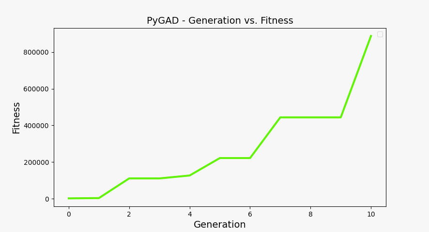
../../../_images/fitness_plot.png — Fitness at each generation plot#

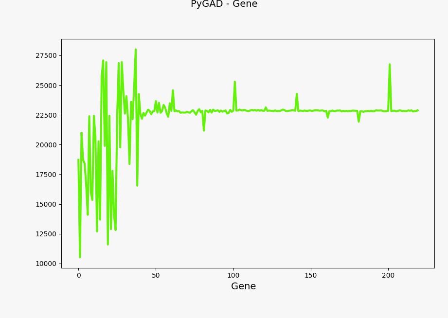
../../../_images/genes.png — Evolution of genes values#

Model storage#

You can store the model in a file for later reuse:

# To save the model data:
from datetime import datetime

# Save the GA instance
# In the filename to save the instance to, do not specify the extension.
formatted_date = datetime.now().strftime("%d-%m-%y")
filename = f"ml_ga_beam_{formatted_date}"
ga_instance.save(filename=filename)

Load the model:

# Load the saved GA instance
loaded_ga_instance = pygad.load(filename=filename)

# Plot fitness function again
loaded_ga_instance.plot_fitness()

Simulation on an HPC cluster using SLURM#

The previous steps create the PyMAPDL script. To see the file, you can click this link ml_ga_beam.py.

To run the preceding script in an HPC environment, you must create a Python environment, install the packages, and then run this script.

Log into your HPC cluster. For more information, see Log into the cluster
Create a virtual environment that is accessible from the compute nodes.
```
user@machine:~$ python3 -m venv /home/user/.venv
```
If you have problems when creating the virtual environment or accessing it from the compute nodes, see Submit a PyMAPDL job.
Install the requirements for this example from the requirements.txt file.

Create the bash script job.sh:

#!/bin/bash
#SBATCH --job-name=ml_ga_beam
#SBATCH --time=01:00:00
#SBATCH --time=1:00:00
#SBATCH --partition=%your_partition_name%
#SBATCH --output=output_%j.txt
#SBATCH --error=error_%j.txt

# Commands to run
echo "Running simulation..."
source /home/user/.venv/bin/activate  # Activate venv
python ml_ga_beam.py
echo "Done"

Remember to replace %your_partition_name% with your cluster partition.

Run the bash script using the sbatch command:
```
sbatch --nodes=1 --ntasks-per-node=10 job.sh
```
The preceding command allocates 10 cores for the job. For optimal performance, this value should be higher than the number of MAPDL instances that the MapdlPool instance is creating.