Harmonic analysis using the frequency-sweep Krylov method#
This example shows how to use the frequency-sweep Krylov method implemented in PyMAPDL. For more information, including the theory behind this method, see Frequency-Sweep Harmonic Analysis via the Krylov Method in the Structural Analysis guide for Mechanical APDL.
Overview#
This example uses the frequency-sweep Krylov method to perform a harmonic analysis on a cylindrical acoustic duct and study the response of the system over a range of frequencies.
The model is a cylindrical acoustic duct with pressure load on one end and output impedance on the other end.
These are the main steps required:
Use the
KrylovSolver.gensubspace()method to generate a Krylov subspace for model reduction in the harmonic analysis.Use the
KrylovSolver.solve()method to reduce the system of equations and solve at each frequency.Use the
KrylovSolver.expand()method to expand the reduced solution back to the FE space.
Perform required imports#
Perform required imports and launch MAPDL.
import os
import numpy as np
import math
import matplotlib.pyplot as plt
from ansys.mapdl.core import launch_mapdl
from ansys.math.core.math import AnsMath

mapdl = launch_mapdl(nproc=4)
mapdl.clear()

# Importing and connecting PyAnsys Math with PyMAPDL
mm = AnsMath(mapdl)
Define parameters#
Define some geometry parameters and analysis settings. As mentioned earlier, the geometry
is a cylinder defined by its radius (cyl_r) and its length (cyl_L). The length
of the duct is such that three complete wavelengths (no_wl) can fit in its length
and can have ten elements per wavelength.
# Constants
pi = np.arccos(-1)
c0 = 340                         # speed of Sound (m/s)

# Materials
rho = 1.2                        # density
c0 = 340                         # speed of Sound
frq = 1000                       # excitation freq   Hz
visco = 0.9                      # viscosity

TP = 1/frq
WL = c0 * TP
no_wl = 3                        # no of wavelengths in space

cyl_L = no_wl * WL               # length of duct
cyl_r = 0.025 * cyl_L            # cross section of duct

nelem_wl = 10                    # no of elements per wavelength
tol_elem = nelem_wl * no_wl      # total number of elements across length
Define element type and materials#
Assign fluid medium (air) properties to the duct. This example
uses Fluid 220 (Keyopt(2)=1) with one degree of freedom per node (pressure),
with no FSI interface in the element.
mapdl.prep7()

mapdl.et(1,'FLUID220', kop2=1)   # uncoupled acoustic element without FSIs
mapdl.mp("DENS", 1, rho)
mapdl.mp("SONC", 1, c0)
mapdl.mp("VISC", 1, visco)
Define geometry#
Create a cylinder of the required dimensions and split it into four segments for uniform generation of the mesh in each segment.
# Set back to default
mapdl.csys(0)

# Rotate working plane for the cylinder generation
mapdl.wpcsys(-1)
mapdl.wprota(thzx=90)

# Generate a circular area with a specified radius
mapdl.cyl4(0, 0, cyl_r)

mapdl.wpcsys(-1)

# Extrude the circular area to generate a cylinder of specified length
mapdl.vext("ALL", dx=cyl_L)

# Split the cylinder into four segments to create a more uniform mesh
mapdl.vsbw("ALL", keep='DELETE')
mapdl.wprota(thzx=90)
mapdl.vsbw("ALL", keep='DELETE')

mapdl.wpcsys(-1)

# Create a component with the created volume
mapdl.cm('cm1', 'volu')
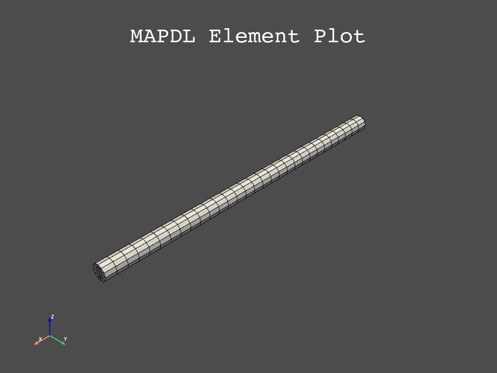
Create mesh#
Create the mesh and plot the FE model.
# Select material and type
mapdl.mat(1)
mapdl.type(1)

# Select volume to mesh
mapdl.cmsel("S", "cm1")
To ensure that the volume is divided in tot_elem across its length, assign
a length element size constraint to the longitudinal lines.
# Select lines belonging to the volume
mapdl.aslv()
mapdl.lsla()

# Unselect lines at the top and bottom faces
mapdl.lsel("U", 'loc', 'x', 0)
mapdl.lsel("U", 'loc', 'x', cyl_L)

# Apply length constraint
mapdl.lesize('ALL',ndiv = tol_elem)
mapdl.lsla()

# Mesh
mapdl.vsweep('ALL')
mapdl.allsel()

# Plot the FE model
mapdl.eplot()
Define boundary conditions#
Apply pressure load on one end and output impedance on other end of the acoustic duct.
# Select areas to apply pressure to
mapdl.cmsel("S", "cm1")
mapdl.aslv()
mapdl.asel('R',"EXT")  # select external areas
mapdl.asel('R',"LOC","x",0)
mapdl.nsla('S',1)

# Apply pressure
mapdl.d('ALL','PRES', 1)

# Select nodes on the areas where impedance is to be applied
mapdl.cmsel("S", "cm1")
mapdl.aslv()
mapdl.asel('R',"EXT")
mapdl.asel('R',"LOC","x",cyl_L)
mapdl.nsla("S",1)

# Apply impedance
mapdl.sf("ALL","IMPD",1000)
mapdl.allsel()
Perform modal analysis#
Get the first 10 natural frequency modes of the acoustic duct.
# Modal Analysis
mapdl.slashsolu()
nev = 10 # Get the first 10 modes
output = mapdl.modal_analysis("DAMP", nmode=nev)
mapdl.finish()
mm.free()

k = mm.stiff(fname=f"{mapdl.jobname}.full")
M = mm.mass(fname=f"{mapdl.jobname}.full")
A = mm.mat(k.nrow, nev)
eigenvalues = mm.eigs(nev, k, M, phi=A, fmin=1.0)
The first ten modes are:
Mode number |
Frequency (Hz) |
|---|---|
1 |
83.33 |
2 |
250.00 |
3 |
416.67 |
4 |
583.34 |
5 |
750.03 |
6 |
916.74 |
7 |
1083.49 |
8 |
1250.32 |
9 |
1417.26 |
10 |
1584.36 |
Run harmonic analysis using Krylov method#
Perform the following steps to run the harmonic analysis using the frequency-sweep Krylov method.
Step 1: Generate FULL file and initialize the Krylov class object.
mapdl.run('/SOLU')
mapdl.antype('HARMIC')  # Set options for harmonic analysis
mapdl.hropt('KRYLOV')
mapdl.eqslv('SPARSE')
mapdl.harfrq(0,1000)    # Set beginning and ending frequency
mapdl.nsubst(100)       # Set the number of frequency increments
mapdl.wrfull(1)         # Generate FULL file and stop
mapdl.solve()
mapdl.finish()

dd = mapdl.krylov       # Initialize Krylov class object
Step 2: Generate a Krylov subspace of size/dimension 10 at frequency 500 Hz for model reduction.
Qz = dd.gensubspace(10, 500, check_orthogonality=True)
Obtain the shape of the generated subspace.
>>> print(Qz.shape)
(3240, 10)
Step 3: Reduce the system of equations and solve at each frequency from 0 Hz to 1000 Hz with ramped loading.
Yz = dd.solve(0, 1000, 100, ramped_load=True)
Obtain the shape of the reduced solution generated.
>>> print(Yz.shape)
(10, 100)
Step 4: Expand the reduced solution back to the FE space.
result = dd.expand(residual_computation=True, residual_algorithm="l2", return_solution = True)
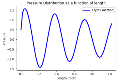
Plot the pressure distribution as a function of length#
Plot the pressure distribution over the length of the duct on nodes where Y, Z coordinates are zero.
# Select all nodes with Z and Y coordinate 0
mapdl.nsel("S", "LOC", "Z", 0)
mapdl.nsel("R", "LOC", "Y", 0)
mapdl.cm("node_comp", "NODES")
comp = mapdl.cmsel("S", "node_comp")
nodes = mapdl.db.nodes
ind, coords, angles = nodes.all_asarray()
Load the last result substep to get the pressure for each of the selected nodes.
x_data = []
y_data = []
substep_index = 99

def get_pressure_at(node, step=1):
    """Get pressure at a given node at a given step (by default first step)"""
    index_num = np.where(result[step]['node'] == node)
    return result[step][index_num]

for each_node, loc in zip(ind, coords):
    # Get pressure at the node
    pressure = get_pressure_at(each_node, substep_index)['x'][0]

    # Calculate amplitude at 60 deg
    magnitude = abs(pressure)
    phase = math.atan2(pressure.imag, pressure.real)
    pressure_a = magnitude * np.cos(np.deg2rad(60)+phase)

    # Store result for later plotting
    x_data.append(loc[0])  # X-Coordenate
    y_data.append(pressure_a)  # Nodal pressure at 60 degrees
Sort the results according to the X coordinate.
sorted_x_data, sorted_y_data = zip(*sorted(zip(x_data, y_data)))
Plot the calculated data.
plt.plot(sorted_x_data, sorted_y_data, linewidth= 3.0, color='b', label='Krylov method')

# Name the graph and the x-axis and y-axis
plt.title("Pressure distribution as a function of length")
plt.xlabel("Length coordinate")
plt.ylabel("Pressure")

# Add legend
plt.legend()

# Load the display window
plt.show()
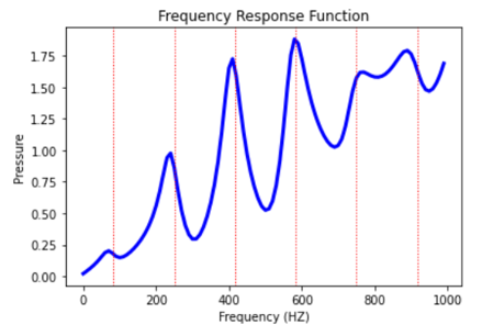
Plot the frequency response function#
Plot the frequency response function of any node along the length of the cylindrical duct. This code plots the frequency response function for a node along 0.2 in the X direction of the duct.
# Pick node closest to 0.2 in X direction, Y&Z = 0
node_number = mapdl.queries.node(0.2, 0, 0)
Get the response of the system for the selected node over a range of frequencies, such as 0 to 1000 Hz.
start_freq = 0
end_freq = 1000
num_steps = 100
step_val = (end_freq - start_freq) / num_steps
dic = {}

for freq in range(0, num_steps):
    pressure = get_pressure_at(node_number, freq)["x"]
    abs_pressure = abs(pressure)

    dic[start_freq] = abs_pressure
    start_freq += step_val
Sort the results.
frf_List = dic.items()
frf_List = sorted(frf_List)
frf_x, frf_y = zip(*frf_List)
Plot the frequency response function for the selected node.
plt.plot(frf_x, frf_y, linewidth=3.0, color="b")

# Plot the natural frequency as vertical lines on the FRF graph
for itr in range(0, 6):
    plt.axvline(
        x=eigenvalues[itr], ymin=0, ymax=2, color="r", linestyle="dotted", linewidth=1
    )

# Name the graph and the x-axis and y-axis
plt.title("Frequency Response Function")
plt.xlabel("Frequency (HZ)")
plt.ylabel("Pressure")

# Load the display window
plt.show()