Basic Thermal Analysis with pyMAPDL

This example demonstrates how you can use MAPDL to create a plate, impose thermal boundary conditions, solve, and plot it all within pyMAPDL.

First, start MAPDL as a service and disable all but error messages.

# sphinx_gallery_thumbnail_number = 2

from ansys.mapdl.core import launch_mapdl

mapdl = launch_mapdl()

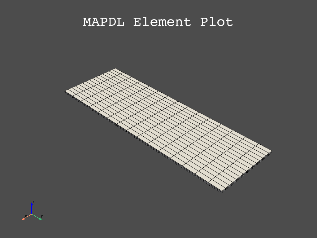
Geometry and Material Properties

Create a simple beam, specify the material properties, and mesh it.

mapdl.prep7()
mapdl.mp("kxx", 1, 45)
mapdl.et(1, 90)
mapdl.block(-0.3, 0.3, -0.46, 1.34, -0.2, -0.2 + 0.02)
mapdl.vsweep(1)
mapdl.eplot()

Boundary Conditions

Set the thermal boundary conditions

mapdl.asel("S", vmin=3)
mapdl.nsla()
mapdl.d("all", "temp", 5)
mapdl.asel("S", vmin=4)
mapdl.nsla()
mapdl.d("all", "temp", 100)
out = mapdl.allsel()

Solve

Solve the thermal static analysis and print the results

mapdl.vsweep(1)
mapdl.run("/SOLU")
print(mapdl.solve())
out = mapdl.finish()

*****  MAPDL SOLVE    COMMAND  *****

 *** NOTE ***                            CP =      39.064   TIME= 18:04:02
 There is no title defined for this analysis.

 *** MAPDL - ENGINEERING ANALYSIS SYSTEM  RELEASE 2023 R1          23.1     ***
 Ansys Mechanical Enterprise
 00000000  VERSION=LINUX x64     18:04:02  AUG 09, 2023 CP=     39.069





                       S O L U T I O N   O P T I O N S

   PROBLEM DIMENSIONALITY. . . . . . . . . . . . .3-D
   DEGREES OF FREEDOM. . . . . . TEMP
   ANALYSIS TYPE . . . . . . . . . . . . . . . . .STATIC (STEADY-STATE)
   GLOBALLY ASSEMBLED MATRIX . . . . . . . . . . .SYMMETRIC

 *** NOTE ***                            CP =      39.070   TIME= 18:04:02
 Present time 0 is less than or equal to the previous time.  Time will
 default to 1.

 *** NOTE ***                            CP =      39.070   TIME= 18:04:02
 The conditions for direct assembly have been met.  No .emat or .erot
 files will be produced.

                      L O A D   S T E P   O P T I O N S

   LOAD STEP NUMBER. . . . . . . . . . . . . . . .     1
   TIME AT END OF THE LOAD STEP. . . . . . . . . .  1.0000
   NUMBER OF SUBSTEPS. . . . . . . . . . . . . . .     1
   STEP CHANGE BOUNDARY CONDITIONS . . . . . . . .    NO
   PRINT OUTPUT CONTROLS . . . . . . . . . . . . .NO PRINTOUT
   DATABASE OUTPUT CONTROLS. . . . . . . . . . . .ALL DATA WRITTEN
                                                  FOR THE LAST SUBSTEP


 SOLUTION MONITORING INFO IS WRITTEN TO FILE= file.mntr


 Range of element maximum matrix coefficients in global coordinates
 Maximum = 13.6474747 at element 449.
 Minimum = 13.6474747 at element 105.

   *** ELEMENT MATRIX FORMULATION TIMES
     TYPE    NUMBER   ENAME      TOTAL CP  AVE CP

        1       450  SOLID90       0.092   0.000203
 Time at end of element matrix formulation CP = 39.178257.

 SPARSE MATRIX DIRECT SOLVER.
  Number of equations =        2606,    Maximum wavefront =     72
  Memory allocated for solver              =     4.813 MB
  Memory required for in-core solution     =     4.639 MB
  Memory required for out-of-core solution =     2.499 MB

 *** NOTE ***                            CP =      39.317   TIME= 18:04:02
 The Sparse Matrix Solver is currently running in the in-core memory
 mode.  This memory mode uses the most amount of memory in order to
 avoid using the hard drive as much as possible, which most often
 results in the fastest solution time.  This mode is recommended if
 enough physical memory is present to accommodate all of the solver
 data.
 Sparse solver maximum pivot= 29.5686693 at node 2185 TEMP.
 Sparse solver minimum pivot= 0.585450932 at node 2282 TEMP.
 Sparse solver minimum pivot in absolute value= 0.585450932 at node 2282
 TEMP.

   *** ELEMENT RESULT CALCULATION TIMES
     TYPE    NUMBER   ENAME      TOTAL CP  AVE CP

        1       450  SOLID90       0.043   0.000096

   *** NODAL LOAD CALCULATION TIMES
     TYPE    NUMBER   ENAME      TOTAL CP  AVE CP

        1       450  SOLID90       0.030   0.000066
 *** LOAD STEP     1   SUBSTEP     1  COMPLETED.    CUM ITER =      1
 *** TIME =   1.00000         TIME INC =   1.00000      NEW TRIANG MATRIX


 *** MAPDL BINARY FILE STATISTICS
  BUFFER SIZE USED= 16384
        1.062 MB WRITTEN ON ASSEMBLED MATRIX FILE: file.full
        0.750 MB WRITTEN ON RESULTS FILE: file.rth

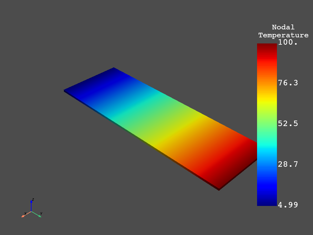
Post-Processing using MAPDL

View the thermal solution of the beam by getting the results directly through MAPDL.

mapdl.post1()
mapdl.set(1, 1)
mapdl.post_processing.plot_nodal_temperature()

Alternatively you could also use the result object that reads in the result file using pyansys

result = mapdl.result
nnum, temp = result.nodal_temperature(0)
# this is the same as pyansys.read_binary(mapdl._result_file)
print(nnum, temp)

[    1     2     3 ... 12715 12716 12717] [ 0.  0.  0. ... nan nan nan]

Stop mapdl

mapdl.exit()