Basic Thermal Analysis with PyMAPDL

This example demonstrates how you can use MAPDL to create a plate, impose thermal boundary conditions, solve, and plot it all within PyMAPDL.

First, start MAPDL as a service and disable all but error messages.

from ansys.mapdl.core import launch_mapdl

mapdl = launch_mapdl()

Geometry and Material Properties

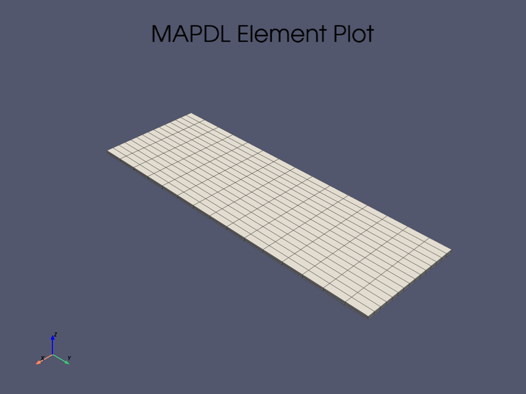
Create a simple beam, specify the material properties, and mesh it.

mapdl.prep7()
mapdl.mp("kxx", 1, 45)
mapdl.et(1, 90)
mapdl.block(-0.3, 0.3, -0.46, 1.34, -0.2, -0.2 + 0.02)
mapdl.vsweep(1)
mapdl.eplot()

Boundary Conditions

Set the thermal boundary conditions

mapdl.asel("S", vmin=3)
mapdl.nsla()
mapdl.d("all", "temp", 5)
mapdl.asel("S", vmin=4)
mapdl.nsla()
mapdl.d("all", "temp", 100)
out = mapdl.allsel()

Solve

Solve the thermal static analysis and print the results

mapdl.vsweep(1)
mapdl.run("/SOLU")
print(mapdl.solve())
out = mapdl.finish()

*** NOTE ***                            CP =      39.879   TIME= 11:10:59
 The automatic domain decomposition logic has selected the MESH domain
 decomposition method with 2 processes per solution.

 *****  MAPDL SOLVE    COMMAND  *****

 *** NOTE ***                            CP =      39.881   TIME= 11:10:59
 There is no title defined for this analysis.

 *** MAPDL - ENGINEERING ANALYSIS SYSTEM  RELEASE                  24.1     ***
 Ansys Mechanical Enterprise Academic Student
 01055371  VERSION=LINUX x64     11:10:59  APR 02, 2024 CP=     39.884





                       S O L U T I O N   O P T I O N S

   PROBLEM DIMENSIONALITY. . . . . . . . . . . . .3-D
   DEGREES OF FREEDOM. . . . . . TEMP
   ANALYSIS TYPE . . . . . . . . . . . . . . . . .STATIC (STEADY-STATE)
   GLOBALLY ASSEMBLED MATRIX . . . . . . . . . . .SYMMETRIC

 *** NOTE ***                            CP =      39.884   TIME= 11:10:59
 Present time 0 is less than or equal to the previous time.  Time will
 default to 1.

 *** NOTE ***                            CP =      39.884   TIME= 11:10:59
 The conditions for direct assembly have been met.  No .emat or .erot
 files will be produced.



     D I S T R I B U T E D   D O M A I N   D E C O M P O S E R

  ...Number of elements: 450
  ...Number of nodes:    2720
  ...Decompose to 2 CPU domains
  ...Element load balance ratio =     1.004


                      L O A D   S T E P   O P T I O N S

   LOAD STEP NUMBER. . . . . . . . . . . . . . . .     1
   TIME AT END OF THE LOAD STEP. . . . . . . . . .  1.0000
   NUMBER OF SUBSTEPS. . . . . . . . . . . . . . .     1
   STEP CHANGE BOUNDARY CONDITIONS . . . . . . . .    NO
   PRINT OUTPUT CONTROLS . . . . . . . . . . . . .NO PRINTOUT
   DATABASE OUTPUT CONTROLS. . . . . . . . . . . .ALL DATA WRITTEN
                                                  FOR THE LAST SUBSTEP


 SOLUTION MONITORING INFO IS WRITTEN TO FILE= file.mntr


 Range of element maximum matrix coefficients in global coordinates
 Maximum = 13.6474747 at element 450.
 Minimum = 13.6474747 at element 105.

   *** ELEMENT MATRIX FORMULATION TIMES
     TYPE    NUMBER   ENAME      TOTAL CP  AVE CP

        1       450  SOLID90       0.029   0.000065
 Time at end of element matrix formulation CP = 39.9380684.

 DISTRIBUTED SPARSE MATRIX DIRECT SOLVER.
  Number of equations =        2606,    Maximum wavefront =     72

  Process memory allocated for solver              =     3.183 MB
  Process memory required for in-core solution     =     3.061 MB
  Process memory required for out-of-core solution =     1.995 MB

  Total memory allocated for solver                =     5.932 MB
  Total memory required for in-core solution       =     5.705 MB
  Total memory required for out-of-core solution   =     3.755 MB

 *** NOTE ***                            CP =      39.990   TIME= 11:10:59
 The Distributed Sparse Matrix Solver is currently running in the
 in-core memory mode.  This memory mode uses the most amount of memory
 in order to avoid using the hard drive as much as possible, which most
 often results in the fastest solution time.  This mode is recommended
 if enough physical memory is present to accommodate all of the solver
 data.
 Distributed sparse solver maximum pivot= 32.7757037 at node 2026 TEMP.
 Distributed sparse solver minimum pivot= 0.721118913 at node 1543 TEMP.
 Distributed sparse solver minimum pivot in absolute value= 0.721118913
 at node 1543 TEMP.

   *** ELEMENT RESULT CALCULATION TIMES
     TYPE    NUMBER   ENAME      TOTAL CP  AVE CP

        1       450  SOLID90       0.024   0.000053

   *** NODAL LOAD CALCULATION TIMES
     TYPE    NUMBER   ENAME      TOTAL CP  AVE CP

        1       450  SOLID90       0.016   0.000035
 *** LOAD STEP     1   SUBSTEP     1  COMPLETED.    CUM ITER =      1
 *** TIME =   1.00000         TIME INC =   1.00000      NEW TRIANG MATRIX


 *** MAPDL BINARY FILE STATISTICS
  BUFFER SIZE USED= 16384
        0.625 MB WRITTEN ON ASSEMBLED MATRIX FILE: file0.full
        0.562 MB WRITTEN ON RESULTS FILE: file0.rth

Post-Processing using MAPDL

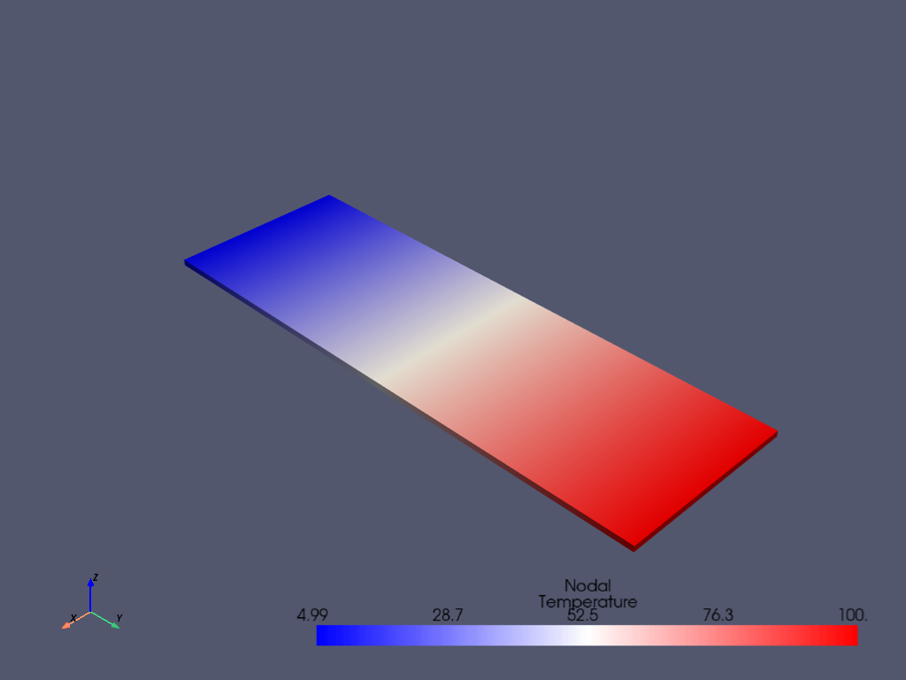
View the thermal solution of the beam by getting the results directly through MAPDL.

mapdl.post1()
mapdl.set(1, 1)
mapdl.post_processing.plot_nodal_temperature()

Alternatively you could also use the result object that reads in the result file using pyansys

result = mapdl.result
nnum, temp = result.nodal_temperature(0)
# this is the same as pyansys.read_binary(mapdl._result_file)
print(nnum, temp)

[    1     2     3 ... 11612 11613 11614] [ 0.  0.  0. ... nan nan nan]

Stop mapdl

mapdl.exit()

/opt/hostedtoolcache/Python/3.10.14/x64/lib/python3.10/site-packages/ansys/mapdl/core/launcher.py:811: UserWarning: The environment variable 'PYMAPDL_START_INSTANCE' is set, hence the argument 'start_instance' is overwritten.
  warnings.warn(