Note
Go to the end to download the full example code.
Basic DPF-Core Usage with PyMAPDL#
This example is adapted from Basic DPF-Core Usage Example and it shows how to open a result file in DPF and do some basic postprocessing.
If you have Ansys 2021 R1 installed, starting DPF is quite easy as DPF-Core takes care of launching all the services that are required for postprocessing Ansys files.
First, import the DPF-Core module as dpf_core and import the
included examples file.
import tempfile

from ansys.dpf import core as dpf

from ansys.mapdl.core import launch_mapdl
from ansys.mapdl.core.examples import vmfiles
Create model#
Running an example from the MAPDL verification manual
mapdl = launch_mapdl()

vm5 = vmfiles["vm5"]
output = mapdl.input(vm5)

print(output)

# If you are working locally, you don't need to perform the following steps
temp_directory = tempfile.gettempdir()

# Downloading RST file to the current folder
rst_path = mapdl.download_result(temp_directory)
/opt/hostedtoolcache/Python/3.12.12/x64/lib/python3.12/site-packages/ansys/tools/common/cyberchannel.py:187: UserWarning:

Starting gRPC client without TLS on 127.0.0.1:21000. This is INSECURE. Consider using a secure connection.


 /INPUT FILE=    LINE=       0
 ANSYS MEDIA REL. 2023R2 (05/12/2023) REF. VERIF. MANUAL: REL. 2023R2

 *** VERIFICATION RUN - CASE VM5                              ***  OPTION=  4


 /SHOW SWITCH PLOTS TO  JPEG        - RASTER MODE.
   *****MAPDL VERIFICATION RUN ONLY*****
     DO NOT USE RESULTS FOR PRODUCTION

          ***** MAPDL ANALYSIS DEFINITION (PREP7) *****

 TITLE=
  VM5, LATERALLY LOADED TAPERED SUPPORT STRUCTURE (QUAD. ELEMENTS)


 C***     MECHANICS OF SOLIDS, CRANDALL AND DAHL, 1959, PAGE 342, PROB. 7.18


 C***          USING PLANE42 ELEMENTS


 PERFORM A STATIC ANALYSIS
  THIS WILL BE A NEW ANALYSIS

 ELEMENT TYPE          1 IS PLANE182     2-D 4-NODE PLANE STRS SOLID
  KEYOPT( 1- 6)=        2      0      3        0      0      0
  KEYOPT( 7-12)=        0      0      0        0      0      0
  KEYOPT(13-18)=        0      0      0        0      0      0

 CURRENT NODAL DOF SET IS  UX    UY
  TWO-DIMENSIONAL MODEL

 REAL CONSTANT SET          1  ITEMS   1 TO   6
    2.0000       0.0000       0.0000       0.0000       0.0000       0.0000

 MATERIAL          1     EX   =  0.3000000E+08

 MATERIAL          1     NUXY =   0.000000

 NODE          1  KCS=      0  X,Y,Z=  25.000       0.0000       0.0000

 NODE          7  KCS=      0  X,Y,Z=  75.000       0.0000       0.0000

 FILL       5 POINTS BETWEEN NODE       1 AND NODE       7
  START WITH NODE       2 AND INCREMENT BY       1

 NODE          8  KCS=      0  X,Y,Z=  25.000      -3.0000       0.0000

 NODE         14  KCS=      0  X,Y,Z=  75.000      -9.0000       0.0000

 FILL       5 POINTS BETWEEN NODE       8 AND NODE      14
  START WITH NODE       9 AND INCREMENT BY       1

 ELEMENT      1       2      1      8      9

 GENERATE       6 TOTAL SETS OF ELEMENTS WITH NODE INCREMENT OF         1
   SET IS SELECTED ELEMENTS IN RANGE         1 TO         1 IN STEPS OF       1

 MAXIMUM ELEMENT NUMBER=         6

 SELECT       FOR ITEM=LOC  COMPONENT=X     BETWEEN  75.000     AND   75.000
   KABS=  0.  TOLERANCE= 0.375000

          2  NODES (OF         14  DEFINED) SELECTED BY  NSEL  COMMAND.

 SPECIFIED CONSTRAINT UX   FOR SELECTED NODES            1 TO          14 BY           1
 REAL=  0.00000000       IMAG=  0.00000000
 ADDITIONAL DOFS=  UY

 ALL SELECT   FOR ITEM=NODE COMPONENT=
  IN RANGE         1 TO         14 STEP          1

         14  NODES (OF         14  DEFINED) SELECTED BY NSEL  COMMAND.

 SPECIFIED NODAL LOAD FY   FOR SELECTED NODES         1 TO        1 BY        1
  REAL= -4000.00000       IMAG=  0.00000000


 ***** ROUTINE COMPLETED *****  CP =         0.000


 *****  MAPDL SOLUTION ROUTINE  *****

 PRINT BASI ITEMS WITH A FREQUENCY OF      1
   FOR ALL APPLICABLE ENTITIES

 /OUTPUT FILE=
Next, open the generated RST file and print out the
Model object.
The Model class helps to
organize access methods for the result by
keeping track of the operators and data sources used by the result
file.
Printing the model displays:
Analysis type
Available results
Size of the mesh
Number of results
If you are working with a remote server, you might need to upload the RST
file before working with it.
Then you can create the DPF Model.
dpf.core.make_tmp_dir_server(dpf.SERVER)

if dpf.SERVER.local_server:
    model = dpf.Model(rst_path)
else:
    server_file_path = dpf.upload_file_in_tmp_folder(rst_path)
    model = dpf.Model(server_file_path)

print(model)
DPF Model
------------------------------
Static analysis
Unit system: Undefined
Physics Type: Mechanical
Available results:
     -  displacement: Nodal Displacement
     -  reaction_force: Nodal Force
     -  elemental_summable_miscellaneous_data: Elemental Elemental Summable Miscellaneous Data
     -  element_nodal_forces: ElementalNodal Element nodal Forces
     -  stress: ElementalNodal Stress
     -  elemental_volume: Elemental Volume
     -  stiffness_matrix_energy: Elemental Energy-stiffness matrix
     -  artificial_hourglass_energy: Elemental Hourglass Energy
     -  thermal_dissipation_energy: Elemental thermal dissipation energy
     -  kinetic_energy: Elemental Kinetic Energy
     -  co_energy: Elemental co-energy
     -  incremental_energy: Elemental incremental energy
     -  elastic_strain: ElementalNodal Strain
     -  thermal_strain: ElementalNodal Thermal Strains
     -  thermal_strains_eqv: ElementalNodal Thermal Strains eqv
     -  swelling_strains: ElementalNodal Swelling Strains
     -  element_euler_angles: ElementalNodal Element Euler Angles
     -  elemental_non_summable_miscellaneous_data: Elemental Elemental Non Summable Miscellaneous Data
     -  structural_temperature: ElementalNodal Structural temperature
------------------------------
DPF  Meshed Region:
  33 nodes
  6 elements
  Unit:
  With shell (2D) elements, shell (3D) elements
------------------------------
DPF  Time/Freq Support:
  Number of sets: 1
Cumulative     Time (s)       LoadStep       Substep
1              1.000000       1              1
Model Metadata#
Specific metadata can be extracted from the model by referencing the
model’s metadata
property. For example, to print only the
result_info:
metadata = model.metadata
print(metadata.result_info)
Static analysis
Unit system: Undefined
Physics Type: Mechanical
Available results:
     -  displacement: Nodal Displacement
     -  reaction_force: Nodal Force
     -  elemental_summable_miscellaneous_data: Elemental Elemental Summable Miscellaneous Data
     -  element_nodal_forces: ElementalNodal Element nodal Forces
     -  stress: ElementalNodal Stress
     -  elemental_volume: Elemental Volume
     -  stiffness_matrix_energy: Elemental Energy-stiffness matrix
     -  artificial_hourglass_energy: Elemental Hourglass Energy
     -  thermal_dissipation_energy: Elemental thermal dissipation energy
     -  kinetic_energy: Elemental Kinetic Energy
     -  co_energy: Elemental co-energy
     -  incremental_energy: Elemental incremental energy
     -  elastic_strain: ElementalNodal Strain
     -  thermal_strain: ElementalNodal Thermal Strains
     -  thermal_strains_eqv: ElementalNodal Thermal Strains eqv
     -  swelling_strains: ElementalNodal Swelling Strains
     -  element_euler_angles: ElementalNodal Element Euler Angles
     -  elemental_non_summable_miscellaneous_data: Elemental Elemental Non Summable Miscellaneous Data
     -  structural_temperature: ElementalNodal Structural temperature
To print the mesh region:
print(metadata.meshed_region)
DPF  Meshed Region:
  33 nodes
  6 elements
  Unit:
  With shell (2D) elements, shell (3D) elements
To print the time or frequency of the results use
time_freq_support:
print(metadata.time_freq_support)
DPF  Time/Freq Support:
  Number of sets: 1
Cumulative     Time (s)       LoadStep       Substep
1              1.000000       1              1
Extracting Displacement Results#
All results of the model can be accessed through the Results
property, which returns the ansys.dpf.core.results.Results
class. This class contains the DPF result operators available to a
specific result file, which are listed when printing the object with
print(results).
Here, the displacement
operator is connected with
DataSources, which
takes place automatically when running
results.displacement().
By default, the displacement
operator is connected to the first result set,
which for this static result is the only result.
results = model.results
displacements = results.displacement()
fields = displacements.outputs.fields_container()

# Finally, extract the data of the displacement field:
disp = fields[0].data
disp
DPFArray([[-4.38851905e-03, -8.90023185e-03,  0.00000000e+00],
          [-6.69683824e-03, -2.11175625e-02,  0.00000000e+00],
          [ 4.17859820e-03, -2.11057663e-02,  0.00000000e+00],
          [ 3.30502628e-03, -8.89049154e-03,  0.00000000e+00],
          [-5.53644478e-03, -1.42612890e-02,  0.00000000e+00],
          [-1.20792265e-03, -2.11145211e-02,  0.00000000e+00],
          [ 3.82436228e-03, -1.42559816e-02,  0.00000000e+00],
          [-4.90502176e-04, -8.89780417e-03,  0.00000000e+00],
          [-2.17801557e-03, -2.15151386e-03,  0.00000000e+00],
          [ 1.82830253e-03, -2.15124124e-03,  0.00000000e+00],
          [-3.27160527e-03, -4.90756375e-03,  0.00000000e+00],
          [ 2.63019818e-03, -4.89004246e-03,  0.00000000e+00],
          [-8.95838911e-05, -2.15503538e-03,  0.00000000e+00],
          [ 0.00000000e+00,  0.00000000e+00,  0.00000000e+00],
          [ 0.00000000e+00,  0.00000000e+00,  0.00000000e+00],
          [-1.07316284e-03, -5.41584305e-04,  0.00000000e+00],
          [ 9.59021573e-04, -5.64429271e-04,  0.00000000e+00],
          [ 0.00000000e+00,  0.00000000e+00,  0.00000000e+00],
          [-1.10106159e-02, -6.60224200e-02,  0.00000000e+00],
          [-1.20838957e-02, -9.90994350e-02,  0.00000000e+00],
          [ 3.61860276e-04, -9.88721453e-02,  0.00000000e+00],
          [ 3.23207196e-03, -6.59380057e-02,  0.00000000e+00],
          [-1.17563515e-02, -8.18061655e-02,  0.00000000e+00],
          [-5.82220244e-03, -9.89754713e-02,  0.00000000e+00],
          [ 2.08036965e-03, -8.18682795e-02,  0.00000000e+00],
          [-3.87518431e-03, -6.59854725e-02,  0.00000000e+00],
          [-8.99066833e-03, -3.98506343e-02,  0.00000000e+00],
          [ 4.27062988e-03, -3.98210573e-02,  0.00000000e+00],
          [-1.00608366e-02, -5.19510806e-02,  0.00000000e+00],
          [ 3.92601832e-03, -5.19563394e-02,  0.00000000e+00],
          [-2.31550786e-03, -3.98370089e-02,  0.00000000e+00],
          [-7.85485340e-03, -2.95981071e-02,  0.00000000e+00],
          [ 4.34038437e-03, -2.95942670e-02,  0.00000000e+00]])
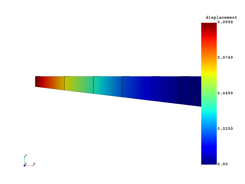
Plot displacements#
You can plot the previous displacement field using:
model.metadata.meshed_region.plot(fields, cpos="xy")

Or using
fields[0].plot(cpos="xy")
This way is particularly useful if you have used ansys.dpf.core.scoping.Scoping
on the mesh or results.
Close session#
Stop MAPDL session.
mapdl.exit()
Total running time of the script: (0 minutes 1.802 seconds)