Analysis of a 2D magnetostatic solenoid

This example shows how to gather and plot results with material discontinuities across elements (Power graphics style) versus the default full average results (Full graphics style).

Description

Mechanical APDL has two averaging methods for presenting results. The following descriptions indicate the primary differences, although other differences exist.

• Full graphics: Presents the entire selected model with node averaged results. In the case of a node shared by two or more elements that have differing materials, the stress field is continuous across the element material boundary (the shared nodes).

• Power graphics: Presents the entire selected model with averaged results within elements of the same material and discontinuous across material boundaries.

This example focuses on material boundaries.

Native PyMAPDL postprocessing is like MAPDL’s Full graphics method with respect to material boundaries.

The geometry of the solenoid is given in Figure 1.

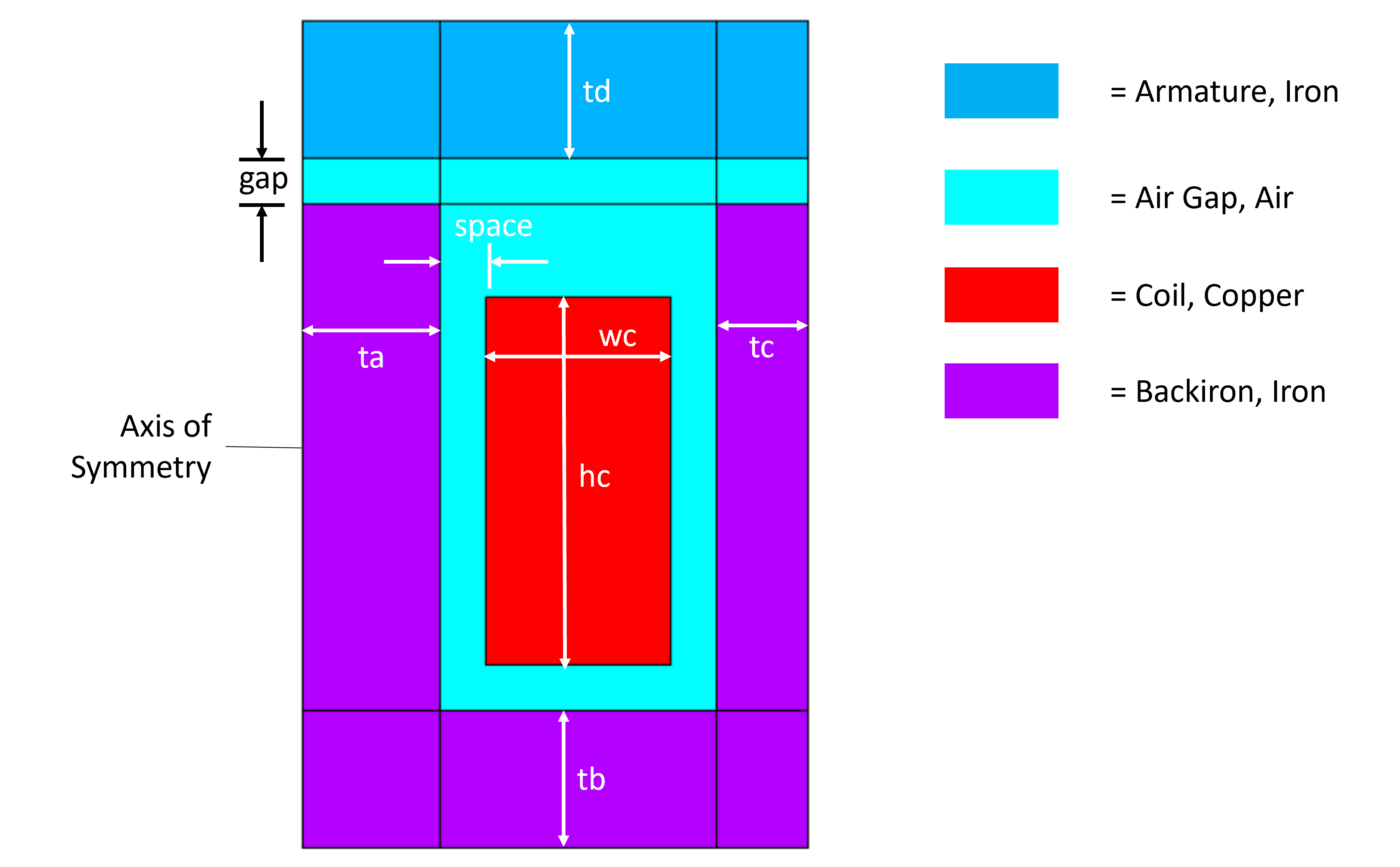
Figure 1: Solenoid geometry description.

Loads and boundary conditions

The coil has a current density applied equal to 650 turns at 1 amp per turn. All exterior nodes have their Z magnetic vector potential set to zero, enforcing a flux parallel condition.

Import modules

In addition to the usual libraries, Matplotlib and PyVista are imported. The MAPDL default contour color style is used so Matplotlib is imported. The Power Graphics style plot is then set up via PyVista.

import numpy as np
import pyvista as pv

from ansys.mapdl.core import launch_mapdl

Launch MAPDL service

mapdl = launch_mapdl()

mapdl.clear()
mapdl.prep7()
mapdl.title("2-D Solenoid Actuator Static Analysis")

TITLE=
 2-D Solenoid Actuator Static Analysis

Set up the FE model

Define parameter values for geometry, loading, and mesh sizing. The model is built in centimeters and is then scaled to meters.

The element type ‘Plane233’ is used for 2D magnetostatic analysis.

mapdl.et(1, "PLANE233")  # Define PLANE233 as element type
mapdl.keyopt(1, 3, 1)  # Use axisymmetric analysis option
mapdl.keyopt(1, 7, 1)  # Condense forces at the corner nodes

ELEMENT TYPE       1 IS PLANE233     AXI 8-NODE MAGNETIC SOLID
  KEYOPT( 1- 6)=        0      0      1        0      0      0
  KEYOPT( 7-12)=        1      0      0        0      0      0
  KEYOPT(13-18)=        0      0      0        0      0      0

 CURRENT NODAL DOF SET IS  AZ
  AXISYMMETRIC MODEL

Set material properties

Units are in the international unit system.

mapdl.mp("MURX", 1, 1)  # Define material properties (permeability), Air
mapdl.mp("MURX", 2, 1000)  # Permeability of backiron
mapdl.mp("MURX", 3, 1)  # Permeability of coil
mapdl.mp("MURX", 4, 2000)  # Permeability of armature

MATERIAL          4     MURX =   2000.000

Set parameters

Set parameters for geometry design.

n_turns = 650  # Number of coil turns
i_current = 1.0  # Current per turn
ta = 0.75  # Model dimensions (centimeters)
tb = 0.75
tc = 0.50
td = 0.75
wc = 1
hc = 2
gap = 0.25
space = 0.25
ws = wc + 2 * space
hs = hc + 0.75
w = ta + ws + tc
hb = tb + hs
h = hb + gap + td
acoil = wc * hc  # Cross-section area of coil (cm**2)
jdens = n_turns * i_current / acoil  # Current density (A/cm**2)

smart_size = 4  # Smart Size Level for Meshing

Create geometry

Create the model geometry.

mapdl.rectng(0, w, 0, tb)  # Create rectangular areas
mapdl.rectng(0, w, tb, hb)
mapdl.rectng(ta, ta + ws, 0, h)
mapdl.rectng(ta + space, ta + space + wc, tb + space, tb + space + hc)
mapdl.aovlap("ALL")
mapdl.rectng(0, w, 0, hb + gap)
mapdl.rectng(0, w, 0, h)
mapdl.aovlap("ALL")
mapdl.numcmp("AREA")  # Compress out unused area numbers

COMPRESS AREA NUMBERS
      MAXIMUM AREA NUMBER COMPRESSED FROM     18 TO     13

Mesh

Set the model mesh.

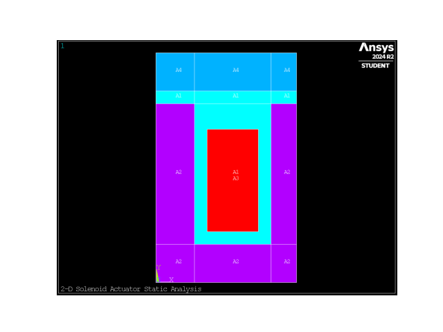
mapdl.asel("S", "AREA", "", 2)  # Assign attributes to coil
mapdl.aatt(3, 1, 1, 0)

mapdl.asel("S", "AREA", "", 1)  # Assign attributes to armature
mapdl.asel("A", "AREA", "", 12, 13)
mapdl.aatt(4, 1, 1)

mapdl.asel("S", "AREA", "", 3, 5)  # Assign attributes to backiron
mapdl.asel("A", "AREA", "", 7, 8)
mapdl.aatt(2, 1, 1, 0)

mapdl.pnum("MAT", 1)  # Turn material numbers on
mapdl.allsel("ALL")

mapdl.aplot(vtk=False)

Mesh

mapdl.smrtsize(smart_size)  # Set smart size meshing
mapdl.amesh("ALL")  # Mesh all areas

GENERATE NODES AND ELEMENTS   IN  ALL  SELECTED AREAS
    ** AREA     1 MESHED WITH      38 QUADRILATERALS,        0 TRIANGLES **
    ** AREA     2 MESHED WITH      50 QUADRILATERALS,        0 TRIANGLES **
    ** AREA     3 MESHED WITH      38 QUADRILATERALS,        0 TRIANGLES **
    ** AREA     4 MESHED WITH      55 QUADRILATERALS,        0 TRIANGLES **
    ** AREA     5 MESHED WITH       54 QUADRILATERALS,        1 TRIANGLES **
    ** AREA     6 MESHED WITH       54 QUADRILATERALS,        0 TRIANGLES **
    ** AREA     7 MESHED WITH       13 QUADRILATERALS,        1 TRIANGLES **
    ** AREA     8 MESHED WITH      16 QUADRILATERALS,        0 TRIANGLES **
    ** AREA     9 MESHED WITH       8 QUADRILATERALS,        0 TRIANGLES **
    ** AREA    10 MESHED WITH       3 QUADRILATERALS,        0 TRIANGLES **
    ** AREA    11 MESHED WITH       4 QUADRILATERALS,        0 TRIANGLES **
    ** AREA    12 MESHED WITH      12 QUADRILATERALS,        0 TRIANGLES **
    ** AREA    13 MESHED WITH      16 QUADRILATERALS,        0 TRIANGLES **

 NUMBER OF AREAS MESHED     =         13
 MAXIMUM NODE NUMBER        =       1158
 MAXIMUM ELEMENT NUMBER     =        363

Scale mesh to meters

Scale the model to be one meter in size.

mapdl.esel("S", "MAT", "", 4)  # Select armature elements
mapdl.cm("ARM", "ELEM")  # Define armature as a component
mapdl.allsel("ALL")
mapdl.arscale(na1="all", rx=0.01, ry=0.01, rz=1, imove=1)  # Scale model to MKS (meters)
mapdl.finish()

***** ROUTINE COMPLETED *****  CP =         2.078

Loads and boundary conditions

Define loads and boundary conditions.

mapdl.slashsolu()

# Apply current density (A/m**2)
mapdl.esel("S", "MAT", "", 3)  # Select coil elements
mapdl.bfe("ALL", "JS", 1, "", "", jdens / 0.01**2)

mapdl.esel("ALL")
mapdl.nsel("EXT")  # Select exterior nodes
mapdl.d("ALL", "AZ", 0)  # Set potentials to zero (flux-parallel)

SPECIFIED CONSTRAINT AZ   FOR SELECTED NODES            1 TO        1158 BY           1
 REAL=  0.00000000       IMAG=  0.00000000

Solve the model

Solve the magnetostatic analysis.

mapdl.allsel("ALL")
mapdl.solve()
mapdl.finish()

FINISH SOLUTION PROCESSING


 ***** ROUTINE COMPLETED *****  CP =         2.181

Postprocessing

Open the result file and read in the last set of results

mapdl.post1()
mapdl.file("file", "rmg")
mapdl.set("last")

USE LAST SUBSTEP ON RESULT FILE  FOR LOAD CASE 0

 SET COMMAND GOT LOAD STEP=     1  SUBSTEP=     1  CUMULATIVE ITERATION=     1
   TIME/FREQUENCY=  1.0000
 TITLE= 2-D Solenoid Actuator Static Analysis

Print the nodal values

print(mapdl.post_processing.nodal_values("b", "x"))

[-0.21167942 -0.08885906  0.04409024 ...  0.          0.
  0.        ]

Create an MAPDL Power Graphics plot of the X-direction magnetic flux

The MAPDL colors are reversed via the rgb command so that the background is white with black text and element edges.

mapdl.graphics("power")
mapdl.rgb("INDEX", 100, 100, 100, 0)
mapdl.rgb("INDEX", 80, 80, 80, 13)
mapdl.rgb("INDEX", 60, 60, 60, 14)
mapdl.rgb("INDEX", 0, 0, 0, 15)

mapdl.edge(1, 1)
mapdl.show("png")
mapdl.pngr("tmod", 0)

mapdl.plnsol("b", "x")
mapdl.show("")

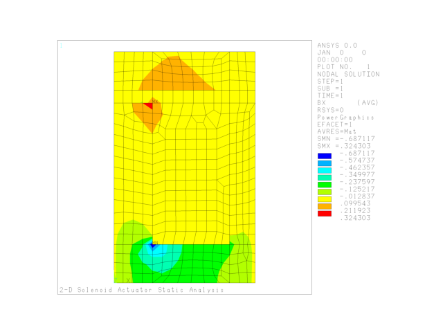
/SHOW SWITCH PLOTS TO  PNG         - RASTER MODE.

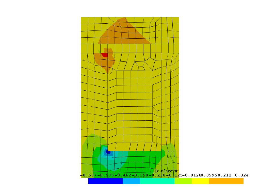
Obtain grid and scalar data

First, obtain the set of unique material IDs in the model

elem_mats = mapdl.mesh.material_type
np.unique(elem_mats)

array([1, 2, 3, 4], dtype=int32)

For each unique material ID, the elements and their nodes are selected. The grids list is appended with the mesh information of just those elements, and the scalars list is appended with the nodal X-direction magnetic flux.

grids = []
scalars = []
for mat in np.unique(elem_mats):
    mapdl.esel("s", "mat", "", mat)
    mapdl.nsle()
    grids.append(mapdl.mesh.grid)
    scalars.append(mapdl.post_processing.nodal_values("b", "x"))
mapdl.allsel()

SELECT ALL ENTITIES OF TYPE= ALL  AND BELOW

If interested print the grids list and perhaps compare to a print of mapdl.mesh.grid

print(grids)
# print(mapdl.mesh.grid)

[UnstructuredGrid (0x7fcc30e9d360)
  N Cells:    69
  N Points:   297
  X Bounds:   0.000e+00, 2.750e-02
  Y Bounds:   7.500e-03, 3.750e-02
  Z Bounds:   0.000e+00, 0.000e+00
  N Arrays:   10, UnstructuredGrid (0x7fcc30e9d780)
  N Cells:    178
  N Points:   623
  X Bounds:   0.000e+00, 2.750e-02
  Y Bounds:   0.000e+00, 3.500e-02
  Z Bounds:   0.000e+00, 0.000e+00
  N Arrays:   10, UnstructuredGrid (0x7fcc30e9c700)
  N Cells:    50
  N Points:   181
  X Bounds:   1.000e-02, 2.000e-02
  Y Bounds:   1.000e-02, 3.000e-02
  Z Bounds:   0.000e+00, 0.000e+00
  N Arrays:   10, UnstructuredGrid (0x7fcc29d8ae60)
  N Cells:    66
  N Points:   235
  X Bounds:   0.000e+00, 2.750e-02
  Y Bounds:   3.750e-02, 4.500e-02
  Z Bounds:   0.000e+00, 0.000e+00
  N Arrays:   10]

Color map and result plot

Because some of the MAPDL contour colors do not have an exact match in the standard Matplotlib color library, an attempt is made to match the color and use the Hex RGBA number value.

For each item in the grids list the grid is added to the plot and 9 contour colors requested using the prior define color map and the same contour legend.

The plot is then shown and it recreates the native plot quite well.

from ansys.mapdl.core.theme import PyMAPDL_cmap

plotter = pv.Plotter()

for i, grid in enumerate(grids):
    plotter.add_mesh(
        grid,
        scalars=scalars[i],
        show_edges=True,
        cmap=PyMAPDL_cmap,
        n_colors=9,
        scalar_bar_args={
            "color": "black",
            "title": "B Flux X",
            "vertical": False,
            "n_labels": 10,
        },
    )

plotter.set_background(color="white")
_ = plotter.camera_position = "xy"
plotter.show()

Exiting MAPDL

mapdl.graphics("FULL")  # Returning to default mode.
mapdl.exit()

/opt/hostedtoolcache/Python/3.10.14/x64/lib/python3.10/site-packages/ansys/mapdl/core/launcher.py:811: UserWarning: The environment variable 'PYMAPDL_START_INSTANCE' is set, hence the argument 'start_instance' is overwritten.
  warnings.warn(