Note

Go to the end to download the full example code

Static analysis of a corner bracket#

This is an example adapted from a classic Ansys APDL tutorial Static Analysis of a Corner Bracket

Problem specification#

Applicable Products:	Ansys Multiphysics, Ansys Mechanical, Ansys Structural
Level of Difficulty:	Easy
Interactive Time Required:	60 to 90 minutes
Discipline:	Structural
Analysis Type:	Linear static
Element Types Used:	PLANE183
Features Demonstrated:	Solid modeling including primitives, boolean operations, and fillets; tapered pressure load deformed shape and stress displays; listing of reaction forces;
Help Resources:	Structural Static Analysis and PLANE183

Problem description#

This is a simple, single-load-step, structural static analysis of a corner angle bracket. The upper-left pin hole is constrained (welded) around its entire circumference, and a tapered pressure load is applied to the bottom of the lower-right pin hole. The US customary system of units is used. The objective is to demonstrate how Mechanical APDL is typical used in an analysis.

Bracket model#

The dimensions of the corner bracket are shown in the following figure. The bracket is made of A36 steel with a Young’s modulus of \(3\cdot10^7\) psi and Poisson’s ratio of \(0.27\).

Bracket image — **Bracket model dimensions**#

Approach and assumptions#

Because the bracket is thin in the z direction (1/2-inch thickness) compared to its x and y dimensions, and because the pressure load acts only in the x-y plane, assume plane stress for the analysis.

The approach is to use solid modeling to generate the 2D model and automatically mesh it with nodes and elements. An alternative approach would be to create the nodes and elements directly.

Launching MAPDL#

from ansys.mapdl.core import launch_mapdl

jobName = "bracket"  # optional
mapdl = launch_mapdl(jobname=jobName)

Build the geometry#

Define rectangles#

There are several ways to create the model geometry within Mechanical APDL, and some are more convenient than others. The first step is to recognize that you can construct the bracket easily with combinations of rectangles and circle primitives.

Select an arbitrary global origin location, and then define the rectangle and circle primitives relative to that origin. For this analysis, use the center of the upper-left hole. Begin by defining a rectangle relative to that location.

The APDL command mapdl.prep7() is used to create a rectangle with X1, X2, Y1, and Y2 dimensions. In PyMAPDL the mapdl() class is used to call the APDL command.

Dimension box 1#

Enter the following:

X1 = 0
X2 = 6
Y1 = -1
Y2 = 1

Or use a Python list to store the dimensions:

box1 = [0, 6, -1, 1]

Dimension box 2#

Enter the following:

box2 = [4, 6, -1, -3]

The mapdl.prep7() command starts the APDL preprocessor to start the build up of the analysis. This is the processor where the model geometry is created.

mapdl.prep7()

*****MAPDL VERIFICATION RUN ONLY*****
     DO NOT USE RESULTS FOR PRODUCTION

          ***** MAPDL ANALYSIS DEFINITION (PREP7) *****

Parameterize as much as possible, taking advantage of Python features such as the Python list or dict class. Good practice would be to have all parameters near or at the top of the input file. However, for this interactive tutorial, they are inline.

# build your cubes
mapdl.rectng(box1[0], box1[1], box1[2], box1[3])

In Python, you can use the * to unpack an object in a function call. For example:

mapdl.rectng(*box2)  # prints the id of the created area

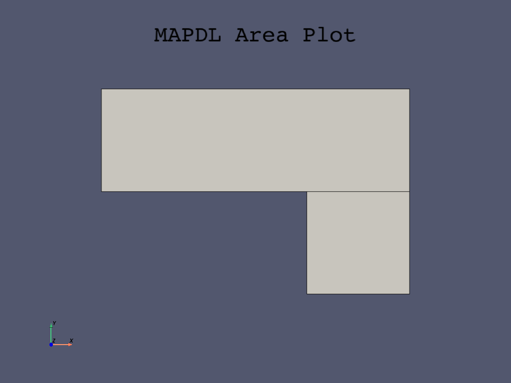
Plot areas#

PyMAPDL plots can be controlled through arguments passed to the different plot methods, such as mapdl.aplot().

The area plot shows both rectangles, which are areas, in the same color. To more clearly distinguish between areas, turn on area numbers. For more information, see the mapdl.aplot() method.

mapdl.aplot(cpos="xy", show_lines=True)

Note

If you download the Jupyter Notebook version of this example, you can take advantage of Jupyter Notebook features. For example, you can right-click a command to display contextual help.

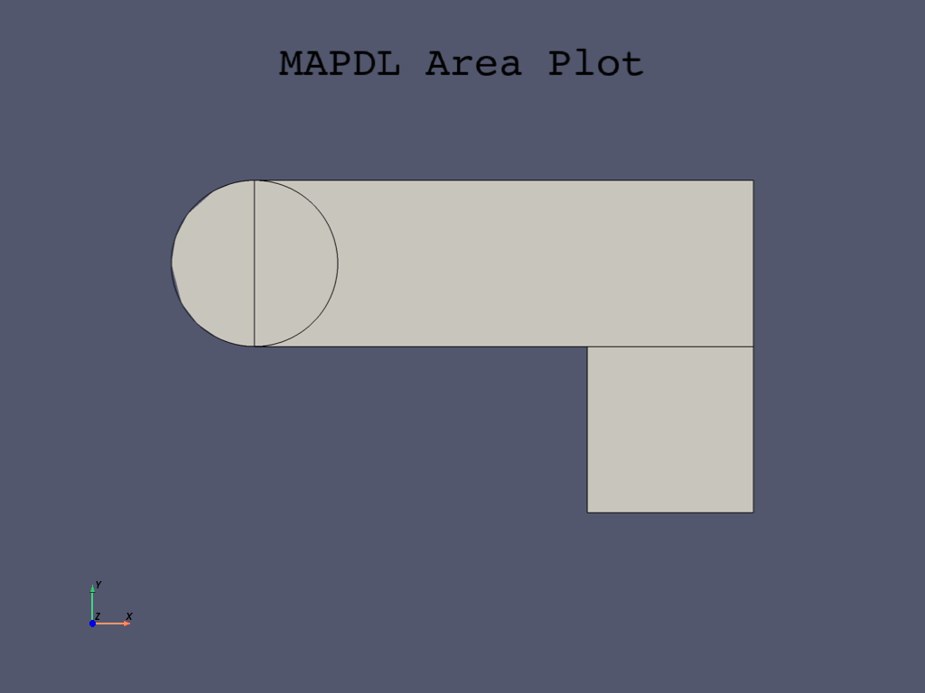
Create first circle#

With the use of logic and Boolean geometrical operations, you can use the original geometric parameters (box1, box2) to locate the circles.

Create the half circle at each end of the bracket. You first create a full circle on each end and then combine the circles and rectangles with a Boolean add operation (discussed in Subtract pin holes from bracket).

The APDL command to create the circles is mapdl.cyl4().

The first circle area is located on the left side at the X,Y location, and its radius is \(1\).

# Create first circle
radius = 1
circle1_X = box1[0]
circle1_Y = (box1[2] + box1[3]) / 2
mapdl.cyl4(circle1_X, circle1_Y, radius)

mapdl.aplot(vtk=True, cpos="xy", show_lines=True)

Create second circle#

Create the second circle at the X,Y location:

circle2_X = (box2[0] + box2[1]) / 2
circle2_Y = box2[3]

Use these parameter values to create the new area with the same radius of \(1\) as the first circle area.

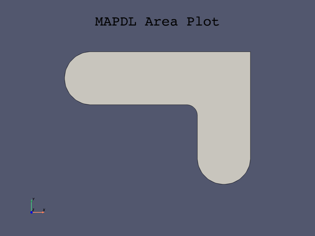
mapdl.cyl4(circle2_X, circle2_Y, radius)
mapdl.aplot(vtk=True, cpos="xy", show_lines=True)

Add areas#

Now that the appropriate pieces of the model (rectangles and circles) are defined, add them together so the model becomes one continuous area. Use the Boolean add operation mapdl.aadd() to add the areas together.

Use the all argument to add all areas.

mapdl.aadd("all")  # Prints the ID of the created area

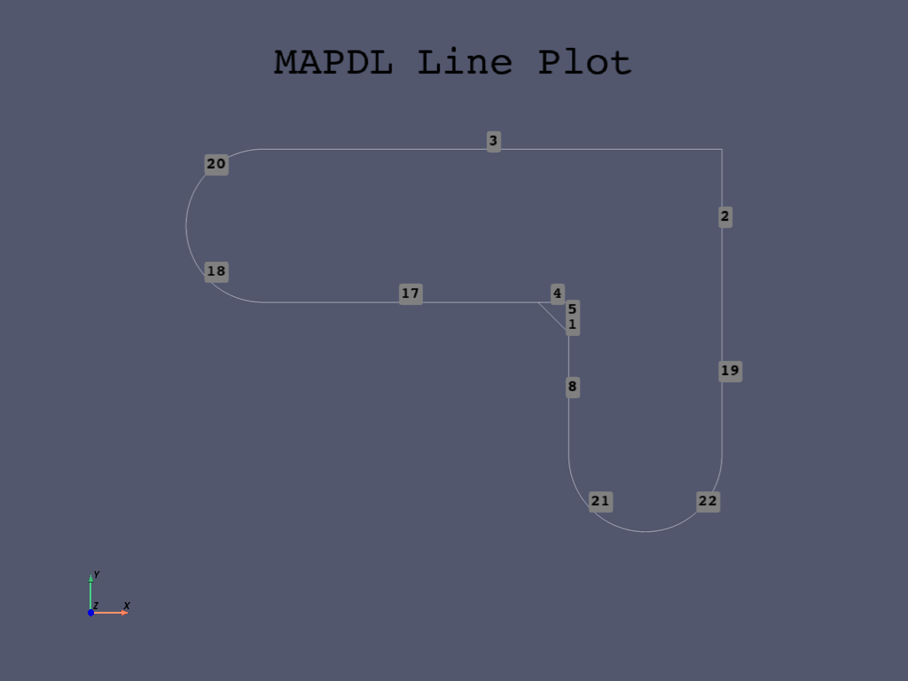
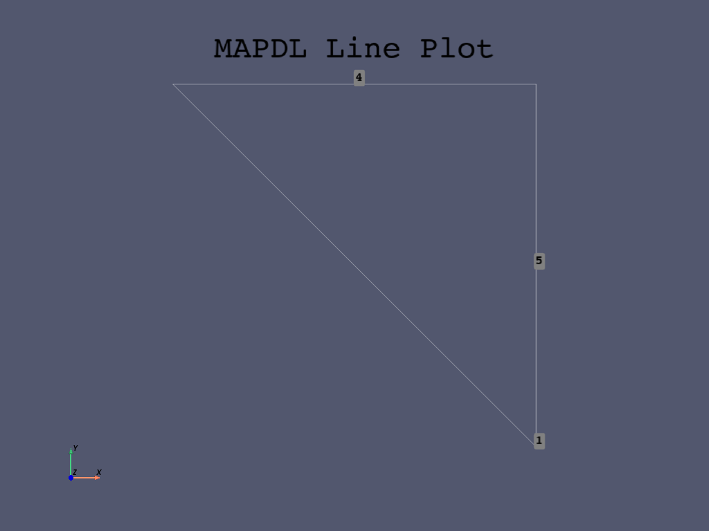
Create line fillet#

The right angle between the two boxes can be improved using a fillet with a radius of \(0.4\). You can do this by selecting the lines around this area and creating the fillet.

Use the APDL mapdl.lsel() method to select lines. Here, the X and Y locations of the lines are used to create the boxes for creating your selection.

After selecting the line, you need to write it to a parameter so you can use it to generate the fillet line. This is done using the mapdl.get() method.

Because you have selected one line, you can use the MAX and NUM arguments for the mapdl.get() method.

Select first line for fillet

line1 = mapdl.lsel("S", "LOC", "Y", box1[2])
l1 = mapdl.get("line1", "LINE", 0, "NUM", "MAX")

If you write the command to a Python parameter (line1), you can use either the APDL parameter l1 or the Python parameter line1 when you create the fillet line.

Select second line for fillet and create Python parameter

line2 = mapdl.lsel("S", "LOC", "X", box2[0])
l2 = mapdl.get("line2", "LINE", 0, "NUM", "MAX")

Once you have both lines selected, you can use the PyMAPDL command mapdl.lfillt() to generate the fillet between the lines.

Note that Python could return a list if more than one line is selected.

Here you use a mix of the APDL parameter as a string line1 and the l2 Python parameter to create the fillet line.

Create fillet line using selected line (parameter names)

fillet_radius = 0.4
mapdl.allsel()
line3 = mapdl.lfillt("line1", l2, fillet_radius)

mapdl.allsel()
mapdl.lplot(vtk=True, cpos="xy")

Create fillet area#

To create the area delineated by line1, line2, and newly created line3, use the mapdl.al() method. The three lines are the input. If you select them all, you can use the 'ALL' argument to create the area.

First you have to reselect the newly created lines in the fillet area. To do this, you can use the fillet_radius parameter and the mapdl.lsel() command.

For the two newly created straight lines, the length is the same as the fillet_radius value. Thus, you can use the length argument with the mapdl.lsel() command.

mapdl.allsel()

# Select lines for the area
mapdl.lsel("S", "LENGTH", "", fillet_radius)

array([4, 5], dtype=int32)

Additionally, you need to get the fillet line itself (line3). You can use the mapdl.lsel() command again with either the 'RADIUS' argument if there is only one line with that radius in the model or more directly use the parameter name of the line. Note the 'A' to additionally select items.

mapdl.lsel("A", "LINE", "", line3)

# plotting ares
mapdl.lplot(vtk=True, cpos="xy", show_line_numbering=True)

Then use mapdl.al() command to create the areas from the lines.

# Create the area
mapdl.al("ALL")  # Prints the ID of the newly created area

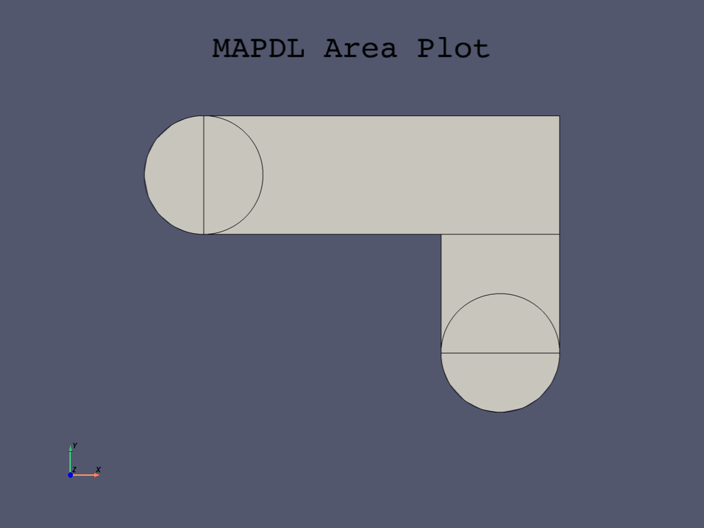
Add areas together#

Append all areas again using the mapdl.aadd() method. Because you have only the two areas to combine, use the 'ALL' argument.

# Add the area to the main area
mapdl.aadd("all")
mapdl.aplot(vtk=True, cpos="xy", show_lines=True)

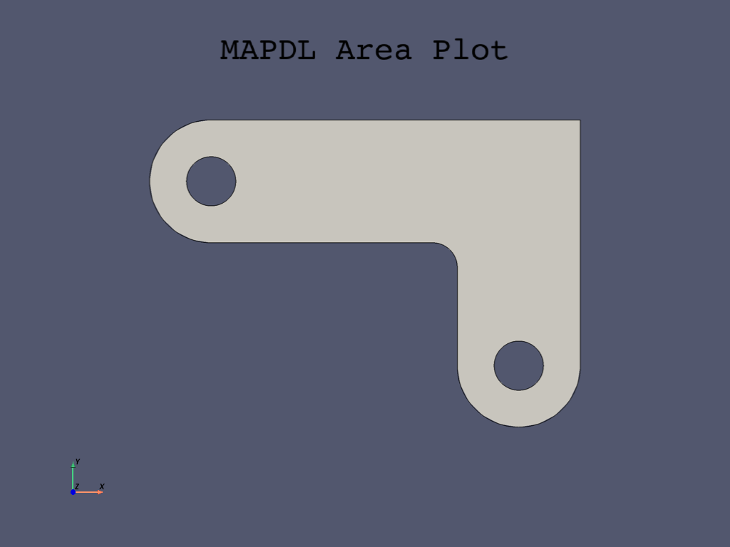
Create first pin hole#

The first pin hole is located at the left side of the first box. Thus, you can use the box dimensions to locate your new circle.

The X value (center) of the pin hole is at the first coordinate of the box1 (X1). The Y value is the average of the two box1 Y values:

# Create the first pinhole
pinhole_radius = 0.4
pinhole1_X = box1[0]
pinhole1_Y = (box1[2] + box1[3]) / 2

pinhole1 = mapdl.cyl4(pinhole1_X, pinhole1_Y, pinhole_radius)

Because you have two pin hole circles, you use the command twice.

Note

Some of these areas are set to parameters to use later in the analysis. This allows you to use the lines to create the areas with the mapdl.asll() command.

Create second pin hole#

The second pin hole is located at the bottom of the second box, so again we can use the box 2 dimensions to locate the circle. For this pinhole the dimensions are:

pinhole2_X = (box2[0] + box2[1]) / 2
pinhole2_Y = box2[3]

pinhole2 = mapdl.cyl4(pinhole2_X, pinhole2_Y, pinhole_radius)
pinhole2_lines = mapdl.asll("S", 0)

Subtract pin holes from bracket#

If you use the mapdl.aplot() command with lines, at this point, you have created two circle areas overlapping the bracket. You can use the mapdl.asba() command, which is the Boolean command to subtract areas, to remove the circles from the bracket.

# Remove pin hole areas from bracket
mapdl.asba("all", pinhole1)
bracket = mapdl.asba("all", pinhole2)
mapdl.aplot(vtk=True, show_lines=True, cpos="xy")

Model definition#

Define material properties#

There is only one material property to define for the bracket, A36 Steel, with given values for the Young’s modulus of elasticity and Poisson’s ratio.

ex = 30e6  # Young's Modulus
prxy = 0.27  # Poisson's ratio

Use the mapdl.mp() command to define material properties in PyMAPDL.

mapdl.mp("EX", 1, ex)
mapdl.mp("PRXY", 1, prxy)

MATERIAL          1     PRXY =  0.2700000

Define element types and options#

You use the mapdl.et() command to select an element .

In any analysis, you select elements from a library of element types and define the appropriate ones for the analysis. In this case, only one element type is used: PLANE183, a 2D, quadratic, structural, higher-order element.

A higher-order element enables you to have a coarser mesh than with lower-order elements while still maintaining solution accuracy. Also, Mechanical APDL generates some triangle-shaped elements in the mesh that would otherwise be inaccurate when using lower-order elements.

Options for PLANE183#

Specify plane stress with thickness as an option for PLANE183. (Thickness is defined as a real constant in Define real constants). Select plane stress with the thickness option for the element behavior. The thickness option is set using the element keyoption 3. For more information, see the PLANE183 element definition in the Ansys Help.

# define a ``PLANE183`` element type with thickness
mapdl.et(1, "PLANE183", kop3=3)

Define real constants#

Assuming plane stress with thickness, enter the thickness as a real constant for PLANE183:

You use the mapdl.r() command to set real constants.

# Set element thickness
thick = 0.5
mapdl.r(1, thick)  # thickness of 0.5 length units)

REAL CONSTANT SET          1  ITEMS   1 TO   6
   0.50000       0.0000       0.0000       0.0000       0.0000       0.0000

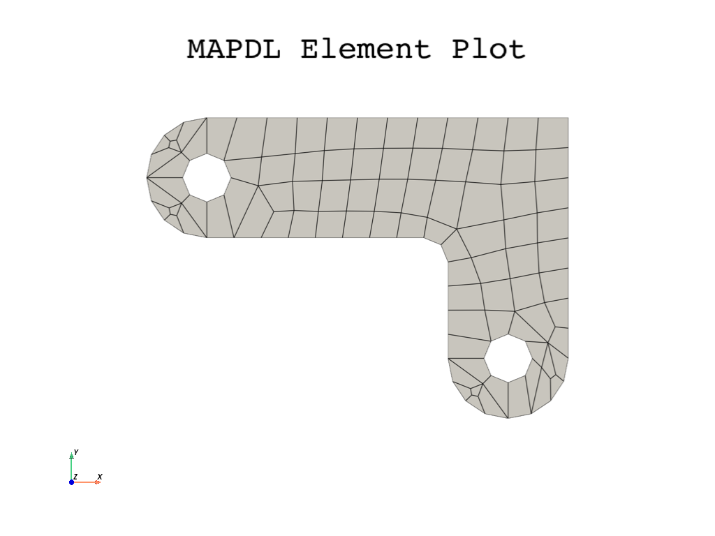
Mesh#

You can mesh the model without specifying mesh-size controls. If you are unsure of how to determine mesh density, you can allow Mechanical APDL to apply a default mesh. For this model, however, you want to specify a global element size to control overall mesh density. Set global size control using the mapdl.esize() command. Set a size of \(0.5\) or a slightly smaller value to improve the mesh.

Mesh the areas using the mapdl.amesh() command. Your mesh may vary slightly from the mesh shown. You may see slightly different results during postprocessing.

Now you can use the mapdl.eplot() command to see the mesh.

element_size = 0.5
mapdl.esize(element_size)
mapdl.amesh(bracket)
mapdl.eplot(
    vtk=True,
    cpos="xy",
    show_edges=True,
    show_axes=False,
    line_width=2,
    background="w",
)

Boundary conditions#

Loading is considered part of the mapdl.solu() command or the solution processor in APDL. But it can be also done in the preprocessor with mapdl.prep7() command.

You can activate the solution processor by calling the mapdl.solution() class, by using the mapdl.slashsolu() command, or by using mapdl.run("/solu") to call the APDL /SOLU command.

mapdl.allsel()
mapdl.solution()

***** ROUTINE COMPLETED *****  CP =         0.000

 *****  MAPDL SOLUTION ROUTINE  *****

Set the analysis type with the mapdl.antype() command.

mapdl.antype("STATIC")

PERFORM A STATIC ANALYSIS
  THIS WILL BE A NEW ANALYSIS

Apply displacement constraints#

This is where you add boundary conditions to the model. First, you want to fix the model by setting a zero displacement at the first pin hole. You can apply displacement constraints directly to lines.

To do this without the graphical interface, you would need to replot the lines. Or you can use Booleans and generate the lines from the pin hole locations/box parameters. By using the parameters that you have created, you can select the lines and fix one end of the bracket.

Pick the four lines around the left-hand hole using the mapdl.lsel() command and the pinehole1 parameters.

bc1 = mapdl.lsel(
    "S", "LOC", "X", pinhole1_X - pinhole_radius, pinhole1_X + pinhole_radius
)
print(f"Number of lines selected : {len(bc1)}")

Number of lines selected : 4

Then for loading, select and apply the boundary condition to the nodes attached to those lines using the mapdl.nsll() command.

fixNodes = mapdl.nsll(type_="S")

Next use the mapdl.d() command to set the displacement to zero (fixed constraint).

# Set up boundary conditions
mapdl.d("ALL", "ALL", 0)  # The 0 is not required since default is zero

# Selecting everything again
mapdl.allsel()

SELECT ALL ENTITIES OF TYPE= ALL  AND BELOW

Apply pressure load#

Apply the tapered pressure load to the bottom-right pin hole. In this case, tapered means varying linearly. When a circle is created in Mechanical APDL, four lines define the perimeter; therefore, apply the pressure to two lines making up the lower half of the circle. Because the pressure tapers from a maximum value (500 psi) at the bottom of the circle to a minimum value (50 psi) at the sides, apply pressure in two separate steps, with reverse tapering values for each line.

p1 = 50
p2 = 500

The Mechanical APDL convention for pressure loading is that a positive load value represents pressure into the surface (compressive).

To pick the line, use the same mapdl.lsel() command used in the previous cell block and then convert the lines to a nodal selection with the mapdl.nsel() command.

Note we have a slightly more complicated picking procedure for the two quarters of the full circle. A method to select the lines would be to select the lower half of the second pinhole circle.

mapdl.lsel("S", "LOC", "Y", pinhole2_Y - pinhole_radius, pinhole2_Y)

array([11, 12], dtype=int32)

Now repick from that selection the lines that are less than the X center of that pin hole.

mapdl.lsel("R", "LOC", "X", 0, pinhole2_X)

mapdl.lplot(vtk=True, cpos="xy")

Once you have the correct line, use the mapdl.sf() command to load the line with the varying surface load.

# Here you load the left side of the lower half of second pin hole.
mapdl.sf("ALL", "PRES", p1, p2)
mapdl.allsel()

SELECT ALL ENTITIES OF TYPE= ALL  AND BELOW

Repeat the procedure for the second pin hole.

mapdl.lsel("S", "LOC", "Y", pinhole2_Y - pinhole_radius, pinhole2_Y)
mapdl.lsel("R", "LOC", "X", pinhole2_X, pinhole2_X + pinhole_radius)

mapdl.lplot(
    vtk=True,
    cpos="xy",
    show_line_numbering=True,
)

mapdl.sf("ALL", "PRES", p2, p1)
mapdl.allsel()

SELECT ALL ENTITIES OF TYPE= ALL  AND BELOW

Solution#

To solve an Ansys FE analysis, the solution processor must be activated, using the mapdl.solution() class or the mapdl.slashsolu() command. This was done a few steps earlier.

The model is ready to be solved using the mapdl.solve() command.

# Solve the model
output = mapdl.solve()
print(output)

*****  MAPDL SOLVE    COMMAND  *****

 *** NOTE ***                            CP =       0.000   TIME= 00:00:00
 There is no title defined for this analysis.

 *** SELECTION OF ELEMENT TECHNOLOGIES FOR APPLICABLE ELEMENTS ***
                ---GIVE SUGGESTIONS ONLY---

 ELEMENT TYPE         1 IS PLANE183 WITH PLANE STRESS OPTION. NO SUGGESTION IS
 AVAILABLE.


   *****MAPDL VERIFICATION RUN ONLY*****
     DO NOT USE RESULTS FOR PRODUCTION

                       S O L U T I O N   O P T I O N S

   PROBLEM DIMENSIONALITY. . . . . . . . . . . . .2-D
   DEGREES OF FREEDOM. . . . . . UX   UY
   ANALYSIS TYPE . . . . . . . . . . . . . . . . .STATIC (STEADY-STATE)
   GLOBALLY ASSEMBLED MATRIX . . . . . . . . . . .SYMMETRIC

 *** NOTE ***                            CP =       0.000   TIME= 00:00:00
 Present time 0 is less than or equal to the previous time.  Time will
 default to 1.

 *** NOTE ***                            CP =       0.000   TIME= 00:00:00
 The imaginary pressure value defined on element 2, face 2 (and possibly
 others) will be not be used for this analysis type, but may be in a
 later analysis.

 *** NOTE ***                            CP =       0.000   TIME= 00:00:00
 The conditions for direct assembly have been met.  No .emat or .erot
 files will be produced.



     D I S T R I B U T E D   D O M A I N   D E C O M P O S E R

  ...Number of elements: 90
  ...Number of nodes:    335
  ...Decompose to 0 CPU domains
  ...Element load balance ratio =     0.000


                      L O A D   S T E P   O P T I O N S

   LOAD STEP NUMBER. . . . . . . . . . . . . . . .     1
   TIME AT END OF THE LOAD STEP. . . . . . . . . .  1.0000
   NUMBER OF SUBSTEPS. . . . . . . . . . . . . . .     1
   STEP CHANGE BOUNDARY CONDITIONS . . . . . . . .    NO
   PRINT OUTPUT CONTROLS . . . . . . . . . . . . .NO PRINTOUT
   DATABASE OUTPUT CONTROLS. . . . . . . . . . . .ALL DATA WRITTEN
                                                  FOR THE LAST SUBSTEP



 Range of element maximum matrix coefficients in global coordinates
 Maximum = 96184869 at element 0.
 Minimum = 31609902.3 at element 0.

   *** ELEMENT MATRIX FORMULATION TIMES
     TYPE    NUMBER   ENAME      TOTAL CP  AVE CP

        1        90  PLANE183      0.000   0.000000
 Time at end of element matrix formulation CP = 0.

 DISTRIBUTED SPARSE MATRIX DIRECT SOLVER.
  Number of equations =         646,    Maximum wavefront =      0
  Memory available (MB) =    0.0    ,  Memory required (MB) =    0.0

 Distributed sparse solver maximum pivot= 0 at node 0 .
 Distributed sparse solver minimum pivot= 0 at node 0 .
 Distributed sparse solver minimum pivot in absolute value= 0 at node 0
 .

   *** ELEMENT RESULT CALCULATION TIMES
     TYPE    NUMBER   ENAME      TOTAL CP  AVE CP

        1        90  PLANE183      0.000   0.000000

   *** NODAL LOAD CALCULATION TIMES
     TYPE    NUMBER   ENAME      TOTAL CP  AVE CP

        1        90  PLANE183      0.000   0.000000
 *** LOAD STEP     1   SUBSTEP     1  COMPLETED.    CUM ITER =      1
 *** TIME =   1.00000         TIME INC =   1.00000      NEW TRIANG MATRIX

Mechanical APDL stores the results of this single-load-step problem in the database and in the results file, Jobname.RST (or Jobname.RTH for thermal or Jobname.RMG for magnetic). The database can contain only one set of results at any given time, so in a multiple-load-step or multiple-substep analysis, Mechanical APDL stores only the final solution in the database.

Mechanical APDL stores all solutions in the results file.

Review the results#

This step represents the beginning of the postprocessing phase.

Note

The results you see may vary slightly from what is shown due to variations in the mesh.

Enter the postprocessor#

The Ansys APDL postprocessor is a separate processor called with the mapdl.post1() command.

mapdl.post1()

FINISH SOLUTION PROCESSING

 ***** ROUTINE COMPLETED *****  CP =         0.000

   *****MAPDL VERIFICATION RUN ONLY*****
     DO NOT USE RESULTS FOR PRODUCTION

          ***** MAPDL RESULTS INTERPRETATION (POST1) *****

 USE LAST SUBSTEP ON RESULT FILE  FOR LOAD CASE 0

 SET COMMAND GOT LOAD STEP=     1  SUBSTEP=     1  CUMULATIVE ITERATION=     1
   TIME/FREQUENCY=  1.0000
 TITLE=

Plot the deformed shape#

Here mapdl.result is used to retrieve the results and for plotting.

# Plot displacement
result = mapdl.result
result_set = 0  # Plotting the first results
disp_fact = 1e10
result.plot_nodal_displacement(
    result_set,
    cpos="xy",
    displacement_factor=5,
    show_displacement=True,
    show_edges=True,
)

Plot the von Mises equivalent stress#

You can also generate stress plots using the mapdl.plot_principal_nodal_stress() command.

result.plot_principal_nodal_stress(
    0,
    "SEQV",
    cpos="xy",
    background="w",
    text_color="k",
    add_text=True,
    show_edges=True,
)

Obtain von Mises stresses.

nnum, stress = result.principal_nodal_stress(0)

# Von Mises stress is the last column in the stress results
von_mises = stress[:, -1]

List reaction solution#

To list the FY reactions forces use the APDL mapdl.prrsol() command which print the constrained node reaction solution.

You can use the to_dataframe command to convert the output to a dataframe for more static print:

reactForces = mapdl.prrsol(lab="FY").to_dataframe(columns=["NODE", "FY"])
print(reactForces)

     NODE       FY
 103.0  21.7590
 104.0   9.8719
 105.0  12.5870
 107.0   1.5168
 108.0  12.2310
 109.0  29.4880
 111.0 -29.8790
 112.0 -10.5920
 113.0  -2.5094
 114.0 -12.4730
115.0  -9.8004
116.0 -22.2000

The values shown are representative and may vary from the values that you obtain. Many other options are available for reviewing results in the general postprocessor. You can see some of these other options in other tutorials, such. as the Ansys tutorial guide.

Exit Mechanical APDL#

Exit Mechanical APDL once you have finished.

mapdl.exit()

Total running time of the script: (0 minutes 5.591 seconds)