Note
Go to the end to download the full example code.
Thermal-structural analysis of exhaust manifold#
This example illustrates how to map results from a CFD analysis and perform a Finite Element (FE) analysis.
Objective#
In this example, we will perform an FE analysis to compute the thermal stresses developed in an exhaust manifold. The manifold is made of structural steel and the temperature distribution in it is obtained from a CFD run. We import this data and map it onto FE mesh to define thermal load at each node using Gaussian interpolation kernel.
Procedure#
Launch MAPDL instance
Import geometry, assign material properties, and generate FE mesh.
Import temperature distribution and map it on FE mesh
Define BCs and use imported temperature distribution to define thermal load.
Solve the model and plot the results of interest.
Additional Packages used#
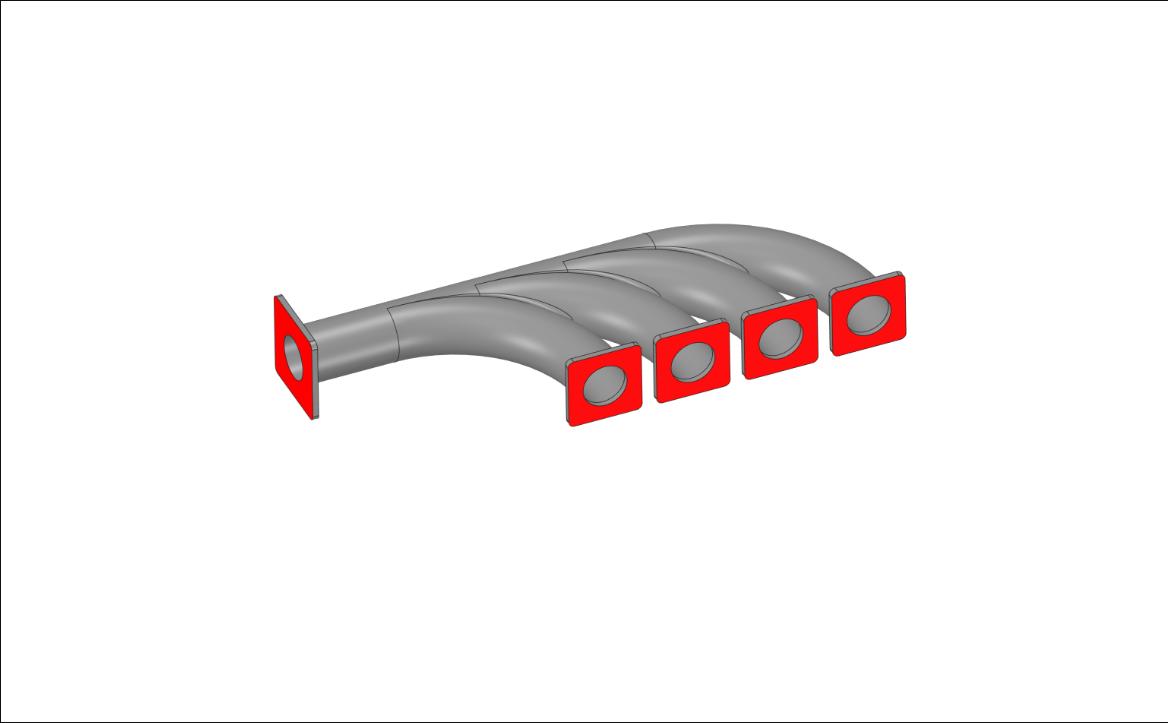
Boundary Conditions#
Highlighted faces are fully constrained.
Import all necessary modules and launch an instance of MAPDL#
import numpy as np
import pandas as pd
import pyvista as pv

from ansys.mapdl.core import launch_mapdl
from ansys.mapdl.core.examples import download_manifold_example_data

# start mapdl
mapdl = launch_mapdl()
print(mapdl)
Mapdl
-----
PyMAPDL Version:     0.73.2
Interface:           grpc
Product:             Ansys Mechanical Enterprise
MAPDL Version:       25.2
Running on:          localhost
                     (127.0.0.1)
Import geometry, assign material properties and generate a mesh.#
# download the necessary files
paths = download_manifold_example_data()
geometry = paths["geometry"]
mapping_data = paths["mapping_data"]

# reset mapdl & import geometry
mapdl.clear()
mapdl.input(geometry)

# Define element attributes
# Second-order tetrahedral elements (SOLID187)
mapdl.prep7()
mapdl.et(1, "SOLID187")

# Define material properties of structural steel
E = 2e11  # Youngs modulus
NU = 0.3  # Poisson's ratio
CTE = 1.2e-5  # Coeff. of thermal expansion
mapdl.mp("EX", 1, E)
mapdl.mp("PRXY", 1, NU)
mapdl.mp("ALPX", 1, CTE)

# Define mesh controls and generate mesh
mapdl.esize(0.0075)
mapdl.vmesh("all")

# Save mesh as VTK object
print(mapdl.mesh)
grid = mapdl.mesh.grid  # save mesh as a VTK object
ANSYS Mesh
  Number of Nodes:              87584
  Number of Elements:           44246
  Number of Element Types:      1
  Number of Node Components:    0
  Number of Element Components: 0
Import and map temperature data to FE mesh#
# Import csv file and save data to a NumPy array
temperature_file = pd.read_csv(mapping_data, sep=",", header=None, low_memory=False)
temperature_data = temperature_file.values # Save data to a NumPy array
nd_temp_data = temperature_data[1:, 1:].astype(float) # Change data type to Float
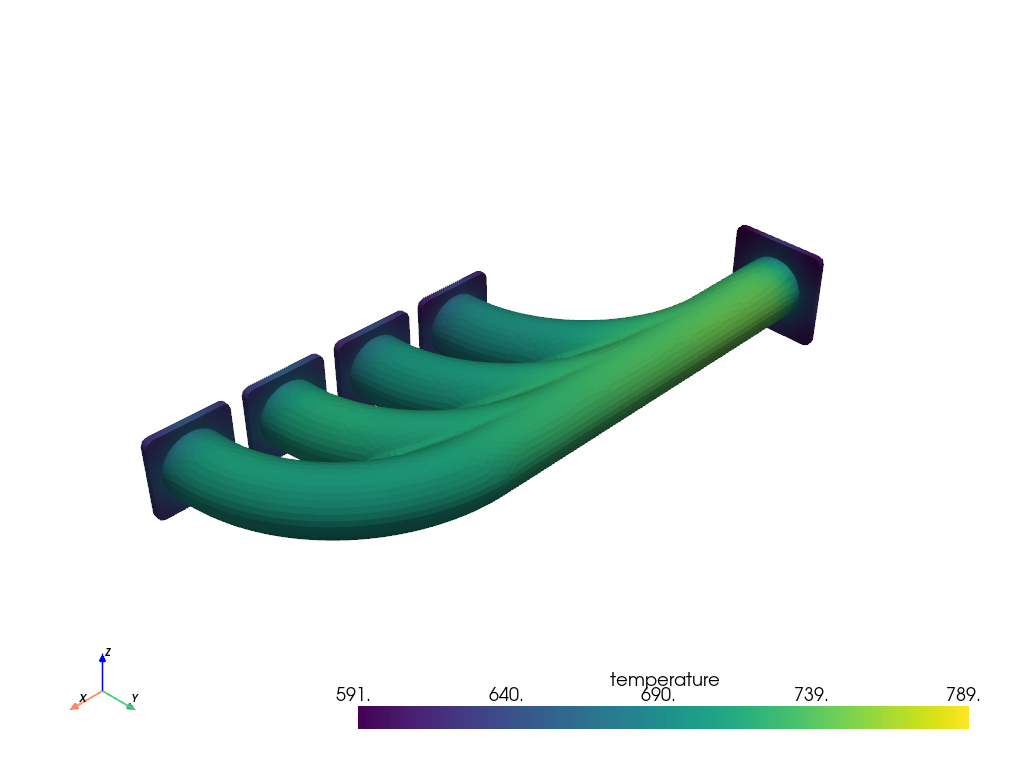
# Map temperature data to FE mesh
# Convert imported data into PolyData format
wrapped = pv.PolyData(nd_temp_data[:, :3]) # Convert NumPy array to PolyData format
wrapped["temperature"] = nd_temp_data[
:, 3
] # Add a scalar variable 'temperature' to PolyData
# Perform data mapping
inter_grid = grid.interpolate(
wrapped,
sharpness=5,
radius=0.0001,
strategy="closest_point",
progress_bar=True,
) # Map the imported data to MAPDL grid
inter_grid.plot(show_edges=False) # Plot the interpolated data on MAPDL grid
temperature_load_val = pv.convert_array(
pv.convert_array(inter_grid.active_scalars)
) # Save temperatures interpolated to each node as NumPy array
node_num = inter_grid.point_data["ansys_node_num"] # Save node numbers as NumPy array
  0%|          [00:00<?]
Interpolating:   0%|          [00:00<?]
Interpolating: 100%|██████████[00:00<00:00]
Interpolating: 100%|██████████[00:00<00:00]
Apply loads and boundary conditions and solve the model#
# Read all nodal coords. to an array & extract the X and Y min. bounds
array_nodes = mapdl.mesh.nodes
Xmin = np.amin(array_nodes[:, 0])
Ymin = np.amin(array_nodes[:, 1])

# Enter /SOLU processor to apply loads and BCs
mapdl.finish()
mapdl.slashsolu()

# Enter non-interactive mode to assign thermal load at each node using imported data
with mapdl.non_interactive:
    for node, temp in zip(node_num, temperature_load_val):
        mapdl.bf(node, "TEMP", temp)
# Use the X and Y min. bounds to select nodes from five surfaces that are to be fixed and created a component and fix all DOFs.
mapdl.nsel("s", "LOC", "X", Xmin)  # Select all nodes whose X coord.=Xmin
mapdl.nsel(
    "a", "LOC", "Y", Ymin
)  # Select all nodes whose Y coord.=Ymin and add to previous selection
mapdl.cm("fixed_nodes", "NODE")  # Create a nodal component 'fixed_nodes'
mapdl.allsel()  # Revert active selection to full model
mapdl.d(
    "fixed_nodes", "all", 0
)  # Impose fully fixed constraint on component created earlier

# Solve the model
output = mapdl.solve()
print(output)
*****  MAPDL SOLVE    COMMAND  *****

 *** WARNING ***                         CP =       0.000   TIME= 00:00:00
 Previous testing revealed that 128 of the 44246 selected elements
 violate shape warning limits.  To review warning messages, please see
 the output or error file, or issue the CHECK command.

 *** NOTE ***                            CP =       0.000   TIME= 00:00:00
 The model data was checked and warning messages were found.
  Please review output or errors file ( ) for these warning messages.

 *** SELECTION OF ELEMENT TECHNOLOGIES FOR APPLICABLE ELEMENTS ***
                ---GIVE SUGGESTIONS ONLY---

 ELEMENT TYPE         1 IS SOLID187. IT IS NOT ASSOCIATED WITH FULLY INCOMPRESSIBLE
 HYPERELASTIC MATERIALS. NO SUGGESTION IS AVAILABLE.


   *****MAPDL VERIFICATION RUN ONLY*****
     DO NOT USE RESULTS FOR PRODUCTION

                       S O L U T I O N   O P T I O N S

   PROBLEM DIMENSIONALITY. . . . . . . . . . . . .3-D
   DEGREES OF FREEDOM. . . . . . UX   UY   UZ
   ANALYSIS TYPE . . . . . . . . . . . . . . . . .STATIC (STEADY-STATE)
   GLOBALLY ASSEMBLED MATRIX . . . . . . . . . . .SYMMETRIC

 *** NOTE ***                            CP =       0.000   TIME= 00:00:00
 Present time 0 is less than or equal to the previous time.  Time will
 default to 1.

 *** NOTE ***                            CP =       0.000   TIME= 00:00:00
 The conditions for direct assembly have been met.  No .emat or .erot
 files will be produced.


     D I S T R I B U T E D   D O M A I N   D E C O M P O S E R

  ...Number of elements: 44246
  ...Number of nodes:    87584
  ...Decompose to 0 CPU domains
  ...Element load balance ratio =     0.000


                      L O A D   S T E P   O P T I O N S

   LOAD STEP NUMBER. . . . . . . . . . . . . . . .     1
   TIME AT END OF THE LOAD STEP. . . . . . . . . .  1.0000
   NUMBER OF SUBSTEPS. . . . . . . . . . . . . . .     1
   STEP CHANGE BOUNDARY CONDITIONS . . . . . . . .    NO
   PRINT OUTPUT CONTROLS . . . . . . . . . . . . .NO PRINTOUT
   DATABASE OUTPUT CONTROLS. . . . . . . . . . . .ALL DATA WRITTEN
                                                  FOR THE LAST SUBSTEP


 Range of element maximum matrix coefficients in global coordinates
 Maximum = 1.875024314E+11 at element 0.
 Minimum = 313199579 at element 0.

   *** ELEMENT MATRIX FORMULATION TIMES
     TYPE    NUMBER   ENAME      TOTAL CP  AVE CP

        1     44246  SOLID187      0.000   0.000000
 Time at end of element matrix formulation CP = 0.

 DISTRIBUTED SPARSE MATRIX DIRECT SOLVER.
  Number of equations =      251874,    Maximum wavefront =      0
  Memory available (MB) =    0.0    ,  Memory required (MB) =    0.0

 Distributed sparse solver maximum pivot= 0 at node 0 .
 Distributed sparse solver minimum pivot= 0 at node 0 .
 Distributed sparse solver minimum pivot in absolute value= 0 at node 0
 .

   *** ELEMENT RESULT CALCULATION TIMES
     TYPE    NUMBER   ENAME      TOTAL CP  AVE CP

        1     44246  SOLID187      0.000   0.000000

   *** NODAL LOAD CALCULATION TIMES
     TYPE    NUMBER   ENAME      TOTAL CP  AVE CP

        1     44246  SOLID187      0.000   0.000000
 *** LOAD STEP     1   SUBSTEP     1  COMPLETED.    CUM ITER =      1
 *** TIME =   1.00000         TIME INC =   1.00000      NEW TRIANG MATRIX
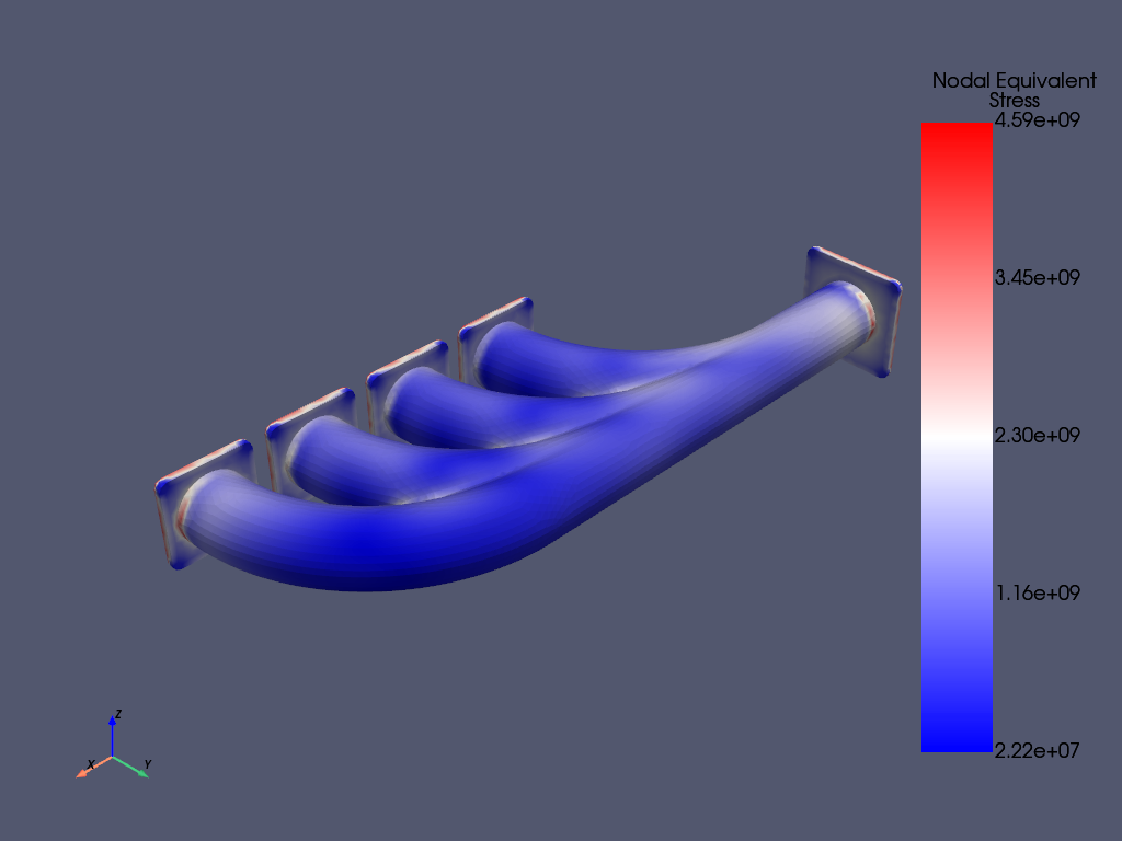
Post-processing#
# Enter post-processor
mapdl.post1()
mapdl.set(1, 1)  # Select first load step
mapdl.post_processing.plot_nodal_eqv_stress()  # Plot equivalent stress
Exit MAPDL instance#
mapdl.exit()
Total running time of the script: (0 minutes 19.739 seconds)