Plotting and Mesh Access

PyMAPDL can load basic IGES geometry for analysis.

This example demonstrates loading basic geometry into MAPDL for analysis and demonstrates how to use the built-in Python specific plotting functionality.

This example also demonstrates some of the more advanced features of PyMAPDL including direct mesh access through VTK.

import numpy as np

from ansys.mapdl import core as pymapdl
from ansys.mapdl.core import examples

mapdl = pymapdl.launch_mapdl()

Load Geometry

Here we download a simple example bracket IGES file and load it into MAPDL. Since igesin must be in the AUX15 process

# note that this method just returns a file path
bracket_file = examples.download_bracket()

# load the bracket and then print out the geometry
mapdl.aux15()
mapdl.igesin(bracket_file)
print(mapdl.geometry)

MAPDL Selected Geometry
Keypoints:  188
Lines:      185
Areas:      73
Volumes:    1

Plotting

PyMAPDL uses VTK and pyvista as a plotting backend to enable remotable (with 2021R1 and newer) interactive plotting. The common plotting methods (kplot, lplot, aplot, eplot, etc.) all have compatible commands that use the ansys.mapdl.core.plotting.general_plotter() function. You can configure this method with a variety of keyword arguments. For example:

mapdl.lplot(
    show_line_numbering=False,
    background="k",
    line_width=3,
    color="w",
    show_axes=False,
    show_bounds=True,
    title="",
    cpos="xz",
)

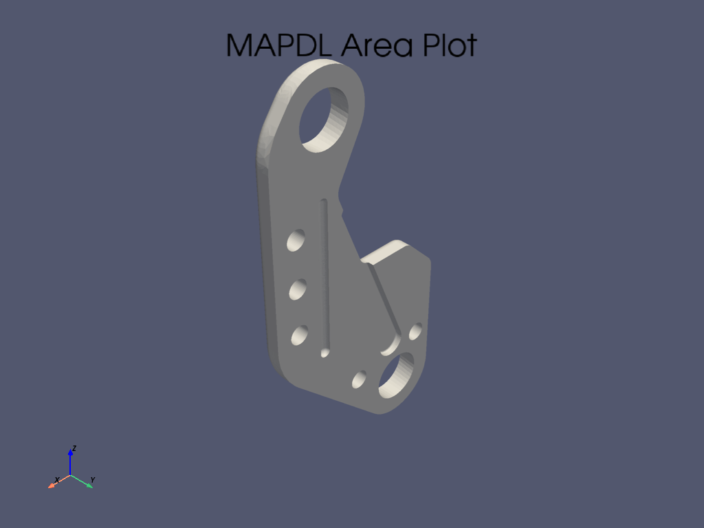
You can also configure a theme to enable consistent plotting across multiple plots. These theme parameters override any unset keyword arguments. For example:

my_theme = pymapdl.MapdlTheme()
my_theme.background = "white"
my_theme.cmap = "jet"  # colormap
my_theme.axes.show = False
my_theme.show_scalar_bar = False

mapdl.aplot(theme=my_theme, quality=8)

Accessesing Element and Nodes Pythonically

PyMAPDL also supports element and nodal plotting using eplot and nplot. First, mesh the bracket using SOLID187 elements. These are well suited to this geometry and the static structural analyses.

# set the preprocessor, element type and size, and mesh the volume
mapdl.prep7()
mapdl.et(1, "SOLID187")
mapdl.esize(0.075)
mapdl.vmesh("all")

# print out the mesh characteristics
print(mapdl.mesh)

ANSYS Mesh
  Number of Nodes:              50565
  Number of Elements:           32115
  Number of Element Types:      1
  Number of Node Components:    0
  Number of Element Components: 0

You can access the underlying finite element mesh as a VTK grid through the mesh.grid attribute.

grid = mapdl.mesh.grid
grid

Header

Data Arrays

UnstructuredGrid Information N Cells 32115 N Points 50565 X Bounds -1.181e+00, 1.181e+00 Y Bounds -2.362e-01, 0.000e+00 Z Bounds -2.394e+00, 2.509e+00 N Arrays 10

Name Field Type N Comp Min Max ansys_node_num Points int32 1 1.000e+00 5.056e+04 vtkOriginalPointIds Points int64 1 0.000e+00 5.056e+04 origid Points int64 1 0.000e+00 5.056e+04 VTKorigID Points int64 1 0.000e+00 5.056e+04 ansys_elem_num Cells int32 1 1.000e+00 3.212e+04 ansys_real_constant Cells int32 1 1.000e+00 1.000e+00 ansys_material_type Cells int32 1 1.000e+00 1.000e+00 ansys_etype Cells int32 1 1.000e+00 1.000e+00 ansys_elem_type_num Cells int32 1 1.870e+02 1.870e+02 vtkOriginalCellIds Cells int64 1 0.000e+00 3.211e+04

This UnstructuredGrid contains a powerful API, including the ability to access the nodes, elements, original node numbers, all with the ability to plot the mesh and add new attributes and data to the grid.

grid.points  # same as mapdl.mesh.nodes

pyvista_ndarray([[-2.03111884e-01, -5.87401575e-02,  4.44426114e-04],
                 [-2.03111884e-01,  0.00000000e+00,  4.44426114e-04],
                 [-2.03111884e-01, -2.93700787e-02,  4.44426114e-04],
                 ...,
                 [-4.51418296e-01, -1.54326811e-01, -6.17372990e-01],
                 [ 4.95126147e-01, -8.12234933e-02,  1.09901235e+00],
                 [-3.92050102e-01, -1.86903380e-01, -2.85033703e-01]])

cell representation in VTK format

grid.cells

array([   10, 15180, 15181, ..., 21973, 48857, 48856])

Obtain node numbers of the grid

grid.point_data["ansys_node_num"]

pyvista_ndarray([    1,     2,     3, ..., 50563, 50564, 50565],
                dtype=int32)

Save arbitrary data to the grid

# must be sized to the number of points
grid.point_data["my_data"] = np.arange(grid.n_points)
grid.point_data

pyvista DataSetAttributes
Association     : POINT
Active Scalars  : ansys_node_num
Active Vectors  : None
Active Texture  : None
Active Normals  : None
Contains arrays :
    ansys_node_num          int32      (50565,)             SCALARS
    vtkOriginalPointIds     int64      (50565,)
    origid                  int64      (50565,)
    VTKorigID               int64      (50565,)
    my_data                 int64      (50565,)

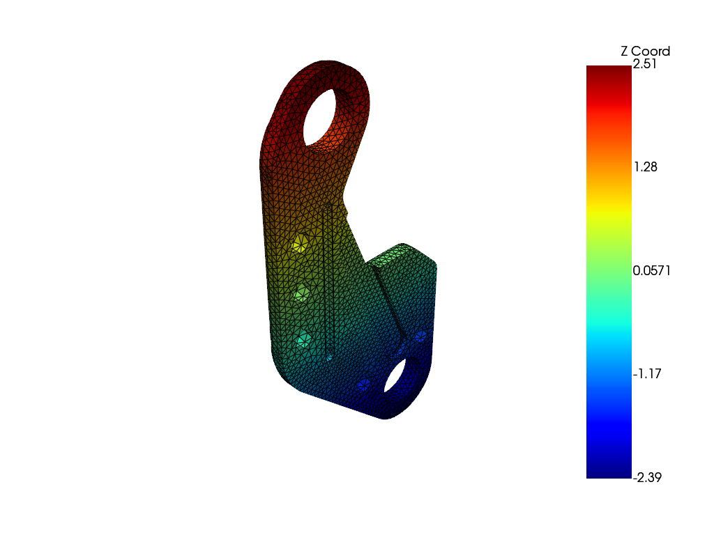
Plot this mesh with scalars of your choosing. You can apply the same MapdlTheme when plotting as it’s compatible with the grid plotter.

# make interesting scalars
scalars = grid.points[:, 2]  # z coordinates

sbar_kwargs = {"color": "black", "title": "Z Coord"}
grid.plot(
    scalars=scalars,
    show_scalar_bar=True,
    scalar_bar_args=sbar_kwargs,
    show_edges=True,
    theme=my_theme,
)

This grid can be also saved to disk in the compact cross-platform VTK format and loaded again with pyvista or ParaView.

..code:: pycon

>>> grid.save('my_mesh.vtk')
>>> import pyvista
>>> imported_mesh = pyvista.read('my_mesh.vtk')

Stop mapdl

mapdl.exit()