Note
Go to the end to download the full example code.
MAPDL 2D Plane Stress Concentration Analysis#
This tutorial shows how you can use PyMAPDL to determine and verify the “stress concentration factor” when modeling using 2D plane elements and then verify this using 3D elements.
First, start MAPDL as a service.
import numpy as np
import plotly.graph_objects as go

from ansys.mapdl.core import launch_mapdl

mapdl = launch_mapdl()
/opt/hostedtoolcache/Python/3.12.13/x64/lib/python3.12/site-packages/ansys/tools/common/cyberchannel.py:201: UserWarning: Starting gRPC client without TLS on 127.0.0.1:21000. This is INSECURE. Consider using a secure connection.
  warn(f"Starting gRPC client without TLS on {target}. This is INSECURE. Consider using a secure connection.")
Element Type and Material Properties#
This example will use PLANE183 elements as a thin plate can be modeled with plane elements provided that KEYOPTION 3 is set to 3 and a thickness is provided.
This example will use SI units.
mapdl.prep7()
mapdl.units("SI")  # SI - International system (m, kg, s, K).

# define a PLANE183 element type with thickness
mapdl.et(1, "PLANE183", kop3=3)
mapdl.r(1, 0.001)  # thickness of 0.001 meters)

# Define a material (nominal steel in SI)
mapdl.mp("EX", 1, 210e9)  # Elastic moduli in Pa (kg/(m*s**2))
mapdl.mp("DENS", 1, 7800)  # Density in kg/m3
mapdl.mp("NUXY", 1, 0.3)  # Poisson's Ratio

# list currently defined material properties
print(mapdl.mplist())
LIST MATERIALS        1 TO        1 BY        1
  PROPERTY= ALL

 MATERIAL NUMBER        1

      TEMP        EX
               0.2100000E+12

      TEMP        NUXY
               0.3000000

      TEMP        DENS
                7800.000
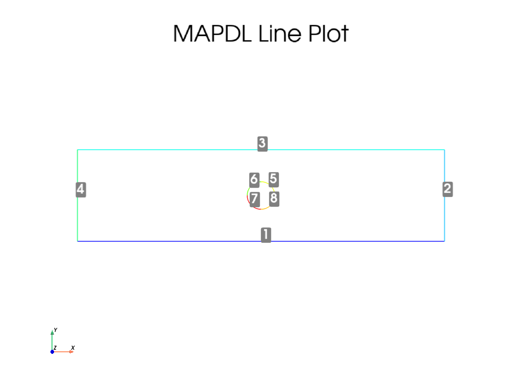
Geometry#
Create a rectangular area with the hole in the middle. To correctly approximate an infinite plate, the maximum stress must occur far away from the edges of the plate. A length to width factor can approximate this.
length = 0.4
width = 0.1

ratio = 0.3  # diameter/width
diameter = width * ratio
radius = diameter * 0.5


# create the rectangle
rect_anum = mapdl.blc4(width=length, height=width)

# create a circle in the middle of the rectangle
circ_anum = mapdl.cyl4(length / 2, width / 2, radius)

# Note how pymapdl parses the output and returns the area numbers
# created by each command.  This can be used to execute a boolean
# operation on these areas to cut the circle out of the rectangle.
plate_with_hole_anum = mapdl.asba(rect_anum, circ_anum)

# finally, plot the lines of the plate
mapdl.lplot(cpos="xy", line_width=3, font_size=26, color_lines=True, background="w")
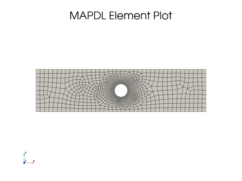
Meshing#
Mesh the plate using a higher density near the hole and a lower
density for the remainder of the plate by setting LESIZE for the
lines nearby the hole and ESIZE for the mesh global size.
Line numbers can be identified through inspection using lplot
# ensure there are at 50 elements around the hole
hole_esize = np.pi * diameter / 50  # 0.0002
plate_esize = 0.01

# increased the density of the mesh at the center
mapdl.lsel("S", "LINE", vmin=5, vmax=8)
mapdl.lesize("ALL", hole_esize, kforc=1)
mapdl.lsel("ALL")

# Decrease the area mesh expansion.  This ensures that the mesh
# remains fine nearby the hole
mapdl.mopt("EXPND", 0.7)  # default 1

mapdl.esize(plate_esize)
mapdl.amesh(plate_with_hole_anum)
mapdl.eplot(
    cpos="xy",
    show_edges=True,
    show_axes=False,
    line_width=2,
    background="w",
)
/opt/hostedtoolcache/Python/3.12.13/x64/lib/python3.12/site-packages/ansys/mapdl/core/mapdl_extended.py:1382: PyVistaFutureWarning: The default value of `algorithm` for the filter
`UnstructuredGrid.extract_surface` will change in the future. It currently defaults to
`'dataset_surface'`, but will change to `None`. Explicitly set the `algorithm` keyword to
silence this warning.
  esurf = self.mesh._grid.linear_copy().extract_surface().clean()
Boundary Conditions#
Fix the left-hand side of the plate in the X direction and set a force of 1 kN in the positive X direction.
# Fix the left-hand side.
mapdl.nsel("S", "LOC", "X", 0)
mapdl.d("ALL", "UX")

# Fix a single node on the left-hand side of the plate in the Y
# direction.  Otherwise, the mesh would be allowed to move in the y
# direction and would be an improperly constrained mesh.
mapdl.nsel("R", "LOC", "Y", width / 2)
assert mapdl.mesh.n_node == 1
mapdl.d("ALL", "UY")

# Apply a force on the right-hand side of the plate.  For this
# example, we select the nodes at the right-most side of the plate.
mapdl.nsel("S", "LOC", "X", length)

# Verify that only the nodes at length have been selected:
assert np.allclose(mapdl.mesh.nodes[:, 0], length)

# Next, couple the DOF for these nodes.  This lets us provide a force
# to one node that will be spread throughout all nodes in this coupled
# set.
mapdl.cp(5, "UX", "ALL")

# Select a single node in this set and apply a force to it
# We use "R" to re-select from the current node group
mapdl.nsel("R", "LOC", "Y", width / 2)
mapdl.f("ALL", "FX", 1000)

# finally, be sure to select all nodes again to solve the entire solution
mapdl.allsel(mute=True)
Solve the Static Problem#
Solve the static analysis
mapdl.solution()
mapdl.antype("STATIC")
output = mapdl.solve()
mapdl.finish()
print(output)
*****  MAPDL SOLVE    COMMAND  *****

 *** NOTE ***                            CP =       0.000   TIME= 00:00:00
 There is no title defined for this analysis.

 *** SELECTION OF ELEMENT TECHNOLOGIES FOR APPLICABLE ELEMENTS ***
                ---GIVE SUGGESTIONS ONLY---

 ELEMENT TYPE         1 IS PLANE183 WITH PLANE STRESS OPTION. NO SUGGESTION IS
 AVAILABLE.


   *****MAPDL VERIFICATION RUN ONLY*****
     DO NOT USE RESULTS FOR PRODUCTION

                       S O L U T I O N   O P T I O N S

   PROBLEM DIMENSIONALITY. . . . . . . . . . . . .2-D
   DEGREES OF FREEDOM. . . . . . UX   UY
   ANALYSIS TYPE . . . . . . . . . . . . . . . . .STATIC (STEADY-STATE)
   GLOBALLY ASSEMBLED MATRIX . . . . . . . . . . .SYMMETRIC

 *** NOTE ***                            CP =       0.000   TIME= 00:00:00
 Present time 0 is less than or equal to the previous time.  Time will
 default to 1.

 *** NOTE ***                            CP =       0.000   TIME= 00:00:00
 The conditions for direct assembly have been met.  No .emat or .erot
 files will be produced.


     D I S T R I B U T E D   D O M A I N   D E C O M P O S E R

  ...Number of elements: 977
  ...Number of nodes:    3083
  ...Decompose to 0 CPU domains
  ...Element load balance ratio =     0.000


                      L O A D   S T E P   O P T I O N S

   LOAD STEP NUMBER. . . . . . . . . . . . . . . .     1
   TIME AT END OF THE LOAD STEP. . . . . . . . . .  1.0000
   NUMBER OF SUBSTEPS. . . . . . . . . . . . . . .     1
   STEP CHANGE BOUNDARY CONDITIONS . . . . . . . .    NO
   PRINT OUTPUT CONTROLS . . . . . . . . . . . . .NO PRINTOUT
   DATABASE OUTPUT CONTROLS. . . . . . . . . . . .ALL DATA WRITTEN
                                                  FOR THE LAST SUBSTEP


            **** CENTER OF MASS, MASS, AND MASS MOMENTS OF INERTIA ****

  CALCULATIONS ASSUME ELEMENT MASS AT ELEMENT CENTROID

  TOTAL MASS =  0.30649

                           MOM. OF INERTIA         MOM. OF INERTIA
  CENTER OF MASS            ABOUT ORIGIN        ABOUT CENTER OF MASS

  XC =  0.20000          IXX =   0.1024E-02      IXX =   0.2576E-03
  YC =  0.49997E-01      IYY =   0.1642E-01      IYY =   0.4156E-02
  ZC =   0.0000          IZZ =   0.1744E-01      IZZ =   0.4414E-02
                         IXY =  -0.3065E-02      IXY =   0.1635E-08
                         IYZ =    0.000          IYZ =    0.000
                         IZX =    0.000          IZX =    0.000


  *** MASS SUMMARY BY ELEMENT TYPE ***

  TYPE      MASS
     1  0.306487

 Range of element maximum matrix coefficients in global coordinates
 Maximum = 1.265076824E+09 at element 0.
 Minimum = 359465553 at element 0.

   *** ELEMENT MATRIX FORMULATION TIMES
     TYPE    NUMBER   ENAME      TOTAL CP  AVE CP

        1       977  PLANE183      0.000   0.000000
 Time at end of element matrix formulation CP = 0.

 DISTRIBUTED SPARSE MATRIX DIRECT SOLVER.
  Number of equations =        6124,    Maximum wavefront =      0
  Memory available (MB) =    0.0    ,  Memory required (MB) =    0.0

 Distributed sparse solver maximum pivot= 0 at node 0 .
 Distributed sparse solver minimum pivot= 0 at node 0 .
 Distributed sparse solver minimum pivot in absolute value= 0 at node 0
 .

   *** ELEMENT RESULT CALCULATION TIMES
     TYPE    NUMBER   ENAME      TOTAL CP  AVE CP

        1       977  PLANE183      0.000   0.000000

   *** NODAL LOAD CALCULATION TIMES
     TYPE    NUMBER   ENAME      TOTAL CP  AVE CP

        1       977  PLANE183      0.000   0.000000
 *** LOAD STEP     1   SUBSTEP     1  COMPLETED.    CUM ITER =      1
 *** TIME =   1.00000         TIME INC =   1.00000      NEW TRIANG MATRIX
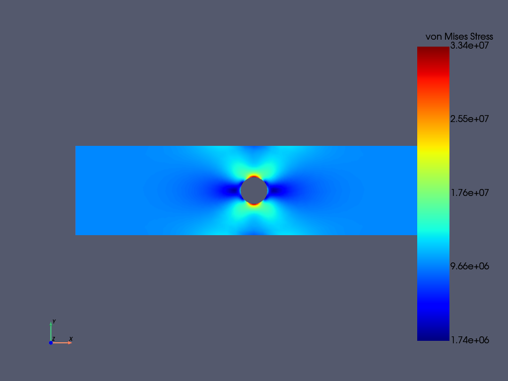
Post-Processing#
The static result can be post-processed both within MAPDL and
outside of MAPDL using pyansys. This example shows how to
extract the von Mises stress and plot it using the pyansys
result reader.
# grab the result from the ``mapdl`` instance
result = mapdl.result
result.plot_principal_nodal_stress(
    0,
    "SEQV",
    lighting=False,
    cpos="xy",
    background="w",
    text_color="k",
    add_text=False,
)

nnum, stress = result.principal_nodal_stress(0)
von_mises = stress[:, -1]  # von-Mises stress is the right most column

# Must use nanmax as stress is not computed at mid-side nodes
max_stress = np.nanmax(von_mises)
/opt/hostedtoolcache/Python/3.12.13/x64/lib/python3.12/site-packages/ansys/mapdl/reader/rst.py:3044: PyVistaFutureWarning: The default value of `algorithm` for the filter
`UnstructuredGrid.extract_surface` will change in the future. It currently defaults to
`'dataset_surface'`, but will change to `None`. Explicitly set the `algorithm` keyword to
silence this warning.
  mesh = grid.extract_surface()
Compute the Stress Concentration#
The stress concentration \(K_t\) is the ratio of the maximum stress at the hole to the far-field stress, or the mean cross sectional stress at a point far from the hole. Analytically, this can be computed with:
\(\sigma_{nom} = \frac{F}{wt}\)
Where
\(F\) is the force
\(w\) is the width of the plate
\(t\) is the thickness of the plate.
Experimentally, this is computed by taking the mean of the nodes at the right-most side of the plate.
# We use nanmean here because mid-side nodes have no stress
mask = result.mesh.nodes[:, 0] == length
far_field_stress = np.nanmean(von_mises[mask])
print("Far field von Mises stress: %e" % far_field_stress)
# Which almost exactly equals the analytical value of 10000000.0 Pa
Far field von Mises stress: 9.999965e+06
Since the expected nominal stress across the cross section of the hole will increase as the size of the hole increases, regardless of the stress concentration, the stress must be adjusted to arrive at the correct stress. This stress is adjusted by the ratio of the width over the modified cross section width.
adj = width / (width - diameter)
stress_adj = far_field_stress * adj

# The stress concentration is then simply the maximum stress divided
# by the adjusted far-field stress.
stress_con = max_stress / stress_adj
print("Stress Concentration: %.2f" % stress_con)
Stress Concentration: 2.34
Batch Analysis#
The above script can be placed within a function to compute the stress concentration for a variety of hole diameters. For each batch, MAPDL is reset and the geometry is generated from scratch.
def compute_stress_con(ratio):
    """Compute the stress concentration for plate with a hole loaded
    with a uniaxial force.
    """
    mapdl.clear("NOSTART")
    mapdl.prep7()
    mapdl.units("SI")  # SI - International system (m, kg, s, K).

    # define a PLANE183 element type with thickness
    mapdl.et(1, "PLANE183", kop3=3)
    mapdl.r(1, 0.001)  # thickness of 0.001 meters)

    # Define a material (nominal steel in SI)
    mapdl.mp("EX", 1, 210e9)  # Elastic moduli in Pa (kg/(m*s**2))
    mapdl.mp("DENS", 1, 7800)  # Density in kg/m3
    mapdl.mp("NUXY", 1, 0.3)  # Poisson's Ratio
    mapdl.emodif("ALL", "MAT", 1)

    # Geometry
    # ~~~~~~~~
    # Create a rectangular area with the hole in the middle
    diameter = width * ratio
    radius = diameter * 0.5

    # create the rectangle
    rect_anum = mapdl.blc4(width=length, height=width)

    # create a circle in the middle of the rectangle
    circ_anum = mapdl.cyl4(length / 2, width / 2, radius)

    # Note how pyansys parses the output and returns the area numbers
    # created by each command.  This can be used to execute a boolean
    # operation on these areas to cut the circle out of the rectangle.
    plate_with_hole_anum = mapdl.asba(rect_anum, circ_anum)

    # Meshing
    # ~~~~~~~
    # Mesh the plate using a higher density near the hole and a lower
    # density for the remainder of the plate

    mapdl.aclear("all")

    # ensure there are at least 100 elements around the hole
    hole_esize = np.pi * diameter / 100  # 0.0002
    plate_esize = 0.01

    # increased the density of the mesh at the center
    mapdl.lsel("S", "LINE", vmin=5, vmax=8)
    mapdl.lesize("ALL", hole_esize, kforc=1)
    mapdl.lsel("ALL")

    # Decrease the area mesh expansion.  This ensures that the mesh
    # remains fine nearby the hole
    mapdl.mopt("EXPND", 0.7)  # default 1

    mapdl.esize(plate_esize)
    mapdl.amesh(plate_with_hole_anum)

    # Boundary Conditions
    # ~~~~~~~~~~~~~~~~~~~
    # Fix the left-hand side of the plate in the X direction
    mapdl.nsel("S", "LOC", "X", 0)
    mapdl.d("ALL", "UX")

    # Fix a single node on the left-hand side of the plate in the Y direction
    mapdl.nsel("R", "LOC", "Y", width / 2)
    assert mapdl.mesh.n_node == 1
    mapdl.d("ALL", "UY")

    # Apply a force on the right-hand side of the plate.  For this
    # example, we select the right-hand side of the plate.
    mapdl.nsel("S", "LOC", "X", length)

    # Next, couple the DOF for these nodes
    mapdl.cp(5, "UX", "ALL")

    # Again, select a single node in this set and apply a force to it
    mapdl.nsel("r", "loc", "y", width / 2)
    mapdl.f("ALL", "FX", 1000)

    # finally, be sure to select all nodes again to solve the entire solution
    mapdl.allsel()

    # Solve the Static Problem
    # ~~~~~~~~~~~~~~~~~~~~~~~~
    mapdl.solution()
    mapdl.antype("STATIC")
    mapdl.solve()
    mapdl.finish()

    # Post-Processing
    # ~~~~~~~~~~~~~~~
    # grab the stress from the result
    result = mapdl.result
    nnum, stress = result.principal_nodal_stress(0)
    von_mises = stress[:, -1]
    max_stress = np.nanmax(von_mises)

    # compare to the "far field" stress by getting the mean value of the
    # stress at the wall
    mask = result.mesh.nodes[:, 0] == length
    far_field_stress = np.nanmean(von_mises[mask])

    # adjust by the cross sectional area at the hole
    adj = width / (width - diameter)
    stress_adj = far_field_stress * adj

    # finally, compute the stress concentration
    return max_stress / stress_adj
Run the batch and record the stress concentration
k_t_exp = []
ratios = np.linspace(0.01, 0.5, 10)
print("    Ratio  : Stress Concentration (K_t)")
for ratio in ratios:
    stress_con = compute_stress_con(ratio)
    print("%10.4f : %10.4f" % (ratio, stress_con))
    k_t_exp.append(stress_con)
Ratio  : Stress Concentration (K_t)
0.0100 :     2.9625
0.0644 :     2.8123
0.1189 :     2.6830
0.1733 :     2.5607
0.2278 :     2.4649
0.2822 :     2.3766
0.3367 :     2.3058
0.3911 :     2.2479
0.4456 :     2.2011
0.5000 :     2.1609
Analytical Comparison#
Stress concentrations are often obtained by referencing tablular results or polynominal fits for a variety of geometries. According to Peterson’s Stress Concentration Factors (ISBN 0470048247), the analytical equation for a hole in a thin plate in uniaxial tension:
\(k_t = 3 - 3.14\frac{d}{h} + 3.667\left(\frac{d}{h}\right)^2 - 1.527\left(\frac{d}{h}\right)^3\)
Where:
\(k_t\) is the stress concentration
\(d\) is the diameter of the circle
\(h\) is the height of the plate
As shown in the following plot, ANSYS matches the known tabular result for this geometry remarkably well using PLANE183 elements. The fit to the results may vary depending on the ratio between the height and width of the plate.
# where ratio is (d/h)
k_t_anl = 3 - 3.14 * ratios + 3.667 * ratios**2 - 1.527 * ratios**3


# Create traces
fig = go.Figure()
fig.add_trace(
    go.Scatter(x=ratios, y=k_t_anl, mode="lines", name=r"$K_t \text{ Analytical}$")
)
fig.add_trace(
    go.Scatter(x=ratios, y=k_t_exp, mode="lines+markers", name=r"$K_t \text{ ANSYS}$")
)

fig.update_layout(
    title="Analytical Comparison",
    xaxis_title="Ratio of Hole Diameter to Width of Plate",
    yaxis_title="Stress Concentration",
)

fig
Stop mapdl#
mapdl.exit()
Total running time of the script: (0 minutes 11.815 seconds)