Note
Go to the end to download the full example code.
Cyclic Analysis#
This example creates a bladed disc using parametric geometry of a cyclic sector and then runs a modal analysis on that cyclic sector. We then post-process the results using the legacy MAPDL reader and finally generate another cyclic model using our parametric modeler.
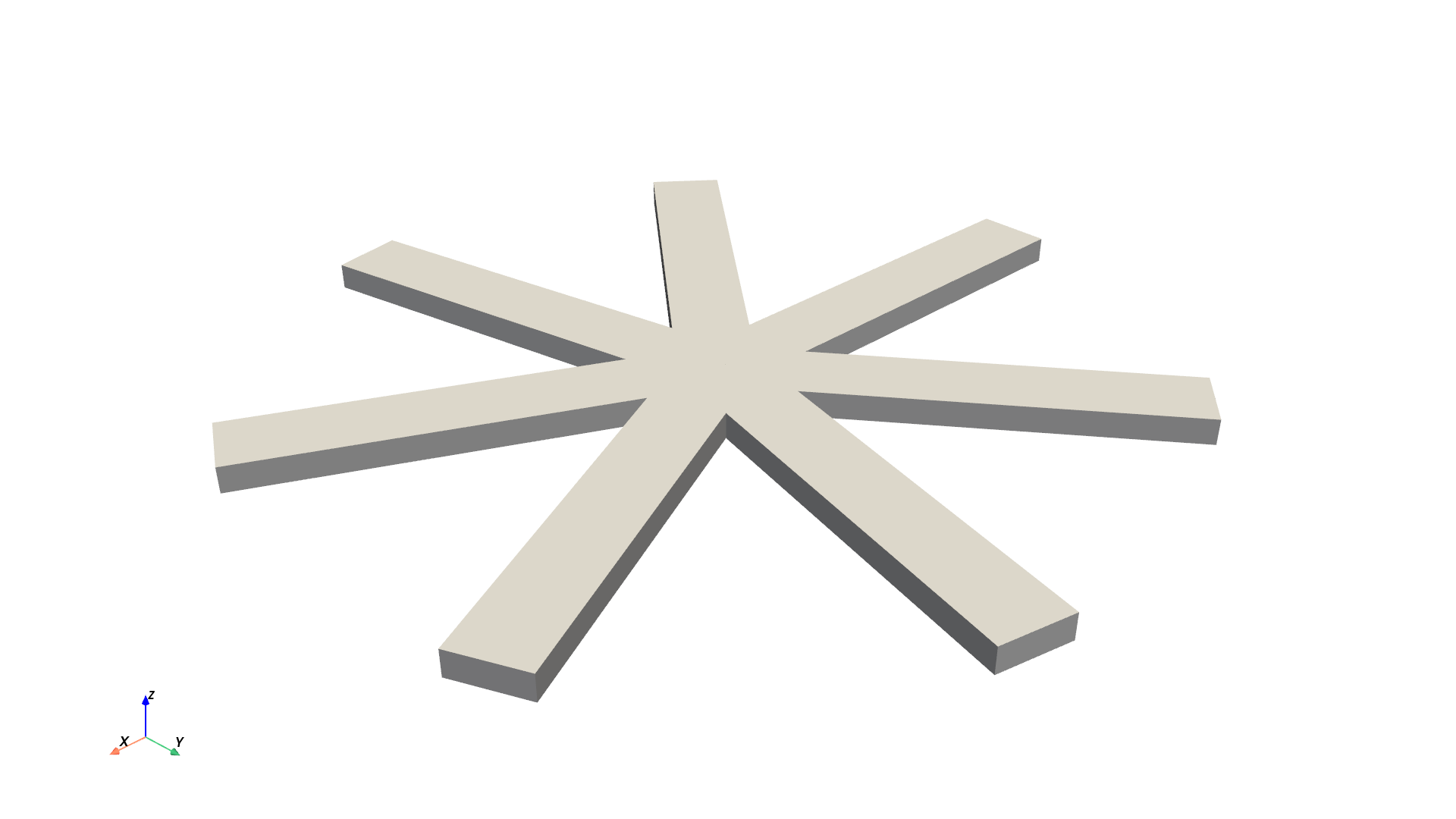
Our first task is to create a simple cyclic model with 7 sectors.
First, start MAPDL as a service.
import numpy as np
import pyvista as pv

from ansys.mapdl.core import launch_mapdl

mapdl = launch_mapdl()
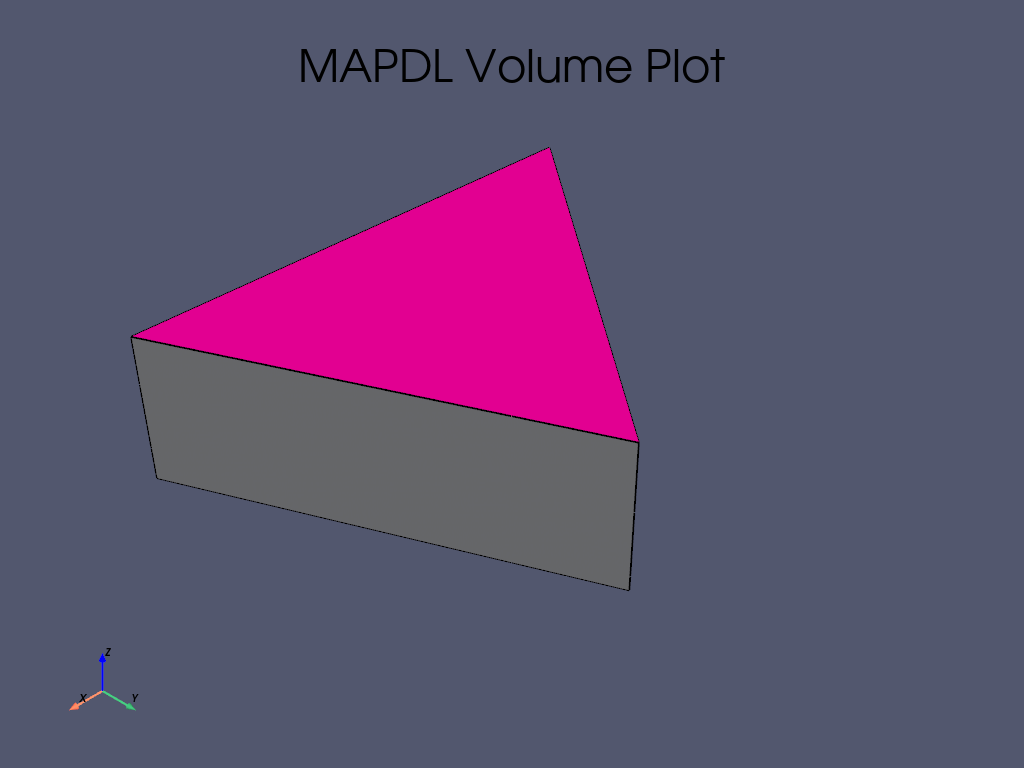
Create the Cyclic Sector#
Create a single “sector” of our cyclic model.
def gen_sector(mapdl, sectors):
"""Generate a single sector within MAPDL."""
# thickness
thickness = 0.003 # meters
arc_end = 2 * np.pi / sectors
arc_cent = arc_end / 2
# radius
rad = 0.01 # M
arc = pv.CircularArc(
[rad, 0, 0],
[np.cos(arc_end) * rad, np.sin(arc_end) * rad, 0],
[0, 0, 0],
)
# interior circle
kp_begin = [rad, 0, 0]
kp_end = [np.cos(arc_end) * rad, np.sin(arc_end) * rad, 0]
kp_center = [0, 0, 0]
# exterior circle in (M)
out_rad = 5.2e-2
# solve for angle to get same arc.length at the end
cent_ang = arc.length / out_rad / 2
# interior circle
kp_beg_outer = [
np.cos(arc_cent - cent_ang) * out_rad,
np.sin(arc_cent - cent_ang) * out_rad,
0,
]
kp_end_outer = [
np.cos(arc_cent + cent_ang) * out_rad,
np.sin(arc_cent + cent_ang) * out_rad,
0,
]
mapdl.prep7()
mapdl.k(0, *kp_center)
mapdl.k(0, *kp_begin)
mapdl.k(0, *kp_end)
mapdl.k(0, *kp_beg_outer)
mapdl.k(0, *kp_end_outer)
# inner arc
mapdl.l(1, 2) # left line
mapdl.l(1, 3) # right line
lnum_inter = mapdl.l(2, 3) # internal line
mapdl.al("all")
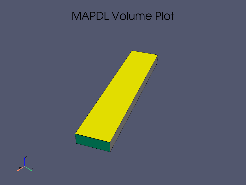
# outer "blade"
lnum = [lnum_inter, mapdl.l(4, 5), mapdl.l(2, 4), mapdl.l(3, 5)]
mapdl.al(*lnum)
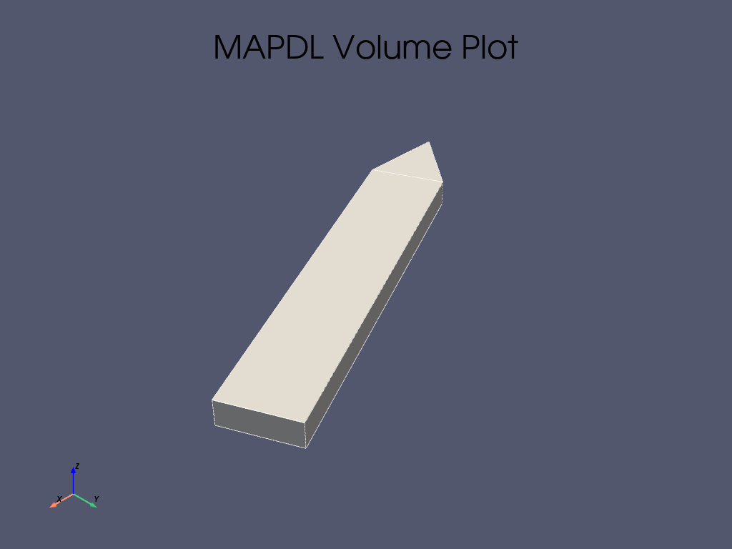
# extrude the model in the Z direction by ``thickness``
mapdl.vext("all", dz=thickness)
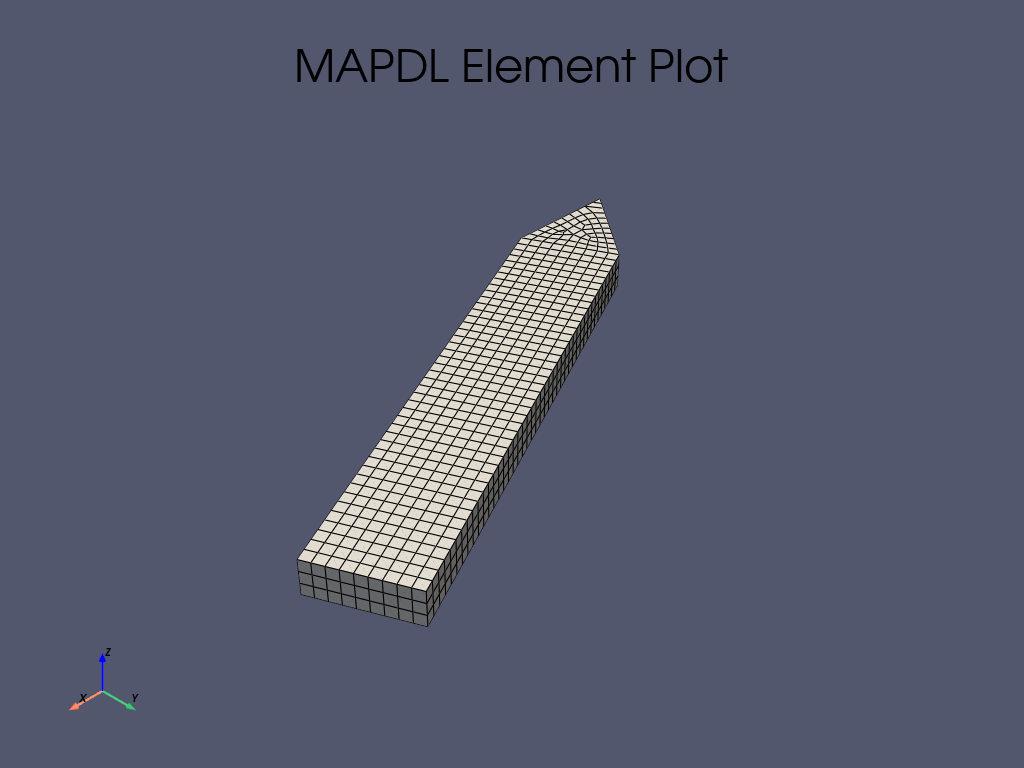
# generate a single sector of a 7 sector model
sectors = 7
gen_sector(mapdl, sectors)
# Volume plot
mapdl.vplot()
Make the Model Cyclic#
Make the model cyclic by running Mapdl.cyclic()
Note how the number of sectors matches
output = mapdl.cyclic()
print(f"Expected Sectors: {sectors}")
print(output)
Expected Sectors: 7
USE EXISTING MODEL FOR CYCLIC SYMMETRY

 ******************************************************
 ****** COMPUTED QUANTITIES ***************************
 ******************************************************
 *  NUMBER OF SECTORS =                  7            *
 *  SECTOR ANGLE =                  51.429            *
 *  CYCLIC COORDINATE SYSTEM =           1            *
 *  EDGE COMPONENTS CONTAIN AREAS                     *
 *  LOW  EDGE COMPONENT = CYCLIC_M01L       MATCHED   *
 *  HIGH EDGE COMPONENT = CYCLIC_M01H                 *
 ******************************************************
Generate the mesh#
Generate the finite element mesh using quadritic hexahedrals, SOLID186.
Apply Material Properties#
# Define a material (nominal steel in SI)
mapdl.mp("EX", 1, 210e9)  # Elastic moduli in Pa (kg/(m*s**2))
mapdl.mp("DENS", 1, 7800)  # Density in kg/m3
mapdl.mp("NUXY", 1, 0.3)  # Poisson's Ratio

# apply it to all elements
mapdl.emodif("ALL", "MAT", 1)
MODIFY ALL SELECTED ELEMENTS TO HAVE MAT = 1
Run the Modal Analysis#
Let’s get the first 10 modes. Note that this will actually compute
(sectors/2)*nmode based on the cyclic boundary conditions.
output = mapdl.modal_analysis(nmode=10, freqb=1)
print(output)
*** NOTE ***                            CP =       0.000   TIME= 00:00:00
 There is no title defined for this analysis.

 *** WARNING ***                         CP =       0.000   TIME= 00:00:00
 No constraints have been defined using the D command.

 GENERATE CYCLIC SYMMETRY CONSTRAINT EQUATIONS

 *** WARNING ***                         CP =       0.000   TIME= 00:00:00
 There is no high edge node in a position to match low edge node 2545
 (location error = 4.55E-04, maximum for all nodes).  Cyclic symmetry
 constraint equations will be generated between the sector edges using
 a mapping procedure similar to the CEINTF command.  This may reduce
 solution accuracy, especially near the sector edges.

 NUMBER OF CONSTRAINT EQUATIONS GENERATED=   363
   (USING THE UNMATCHED NODES ALGORITHM)

 *****  MAPDL SOLVE    COMMAND  *****

 *** SELECTION OF ELEMENT TECHNOLOGIES FOR APPLICABLE ELEMENTS ***
                ---GIVE SUGGESTIONS ONLY---

 ELEMENT TYPE         1 IS SOLID186. KEYOPT(2) IS ALREADY SET AS SUGGESTED.


   *****MAPDL VERIFICATION RUN ONLY*****
     DO NOT USE RESULTS FOR PRODUCTION

                       S O L U T I O N   O P T I O N S

   PROBLEM DIMENSIONALITY. . . . . . . . . . . . .3-D
   CYCLIC SYMMETRY SECTOR ANGLE. . . . . . . . . .   51.429     DEGREES
   DEGREES OF FREEDOM. . . . . . UX   UY   UZ
   ANALYSIS TYPE . . . . . . . . . . . . . . . . .MODAL
      EXTRACTION METHOD. . . . . . . . . . . . . .BLOCK LANCZOS
   NUMBER OF MODES TO EXTRACT. . . . . . . . . . .    10
   USE CYCLIC MODES IN SUBSEQUENT MSUP ANALYSIS. .YES
   SHIFT POINT . . . . . . . . . . . . . . . . . .  1.0000
   GLOBALLY ASSEMBLED MATRIX . . . . . . . . . . .SYMMETRIC
   NUMBER OF MODES TO EXPAND . . . . . . . . . . .    10
   ELEMENT RESULTS CALCULATION . . . . . . . . . .OFF

 *** NOTE ***                            CP =       0.000   TIME= 00:00:00
 The conditions for direct assembly have been met.  No .emat or .erot
 files will be produced.


     D I S T R I B U T E D   D O M A I N   D E C O M P O S E R

  ...Number of elements: 1329
  ...Number of nodes:    7279
  ...Decompose to 0 CPU domains
  ...Element load balance ratio =     0.000


                      L O A D   S T E P   O P T I O N S

   LOAD STEP NUMBER. . . . . . . . . . . . . . . .     1
   CYCLIC SYMMETRY HARMONIC INDEX. . . . . . . . .     0
   THERMAL STRAINS INCLUDED IN THE LOAD VECTOR . .   YES
   PRINT OUTPUT CONTROLS . . . . . . . . . . . . .NO PRINTOUT
   DATABASE OUTPUT CONTROLS. . . . . . . . . . . .ALL DATA WRITTEN


            **** CENTER OF MASS, MASS, AND MASS MOMENTS OF INERTIA ****

  CALCULATIONS ASSUME ELEMENT MASS AT ELEMENT CENTROID

  TOTAL MASS =  0.19205E-01

                           MOM. OF INERTIA         MOM. OF INERTIA
  CENTER OF MASS            ABOUT ORIGIN        ABOUT CENTER OF MASS

  XC =  0.25304E-01      IXX =   0.3686E-05      IXX =   0.7910E-06
  YC =  0.12186E-01      IYY =   0.1533E-04      IYY =   0.2994E-05
  ZC =  0.15000E-02      IZZ =   0.1891E-04      IZZ =   0.3759E-05
                         IXY =  -0.7303E-05      IXY =  -0.1381E-05
                         IYZ =  -0.3510E-06      IYZ =  -0.2541E-20
                         IZX =  -0.7289E-06      IZX =  -0.4553E-20


  *** MASS SUMMARY BY ELEMENT TYPE ***

  TYPE      MASS
     1  0.192050E-01

 Range of element maximum matrix coefficients in global coordinates
 Maximum = 267009791 at element 0.
 Minimum = 160764667 at element 0.

   *** ELEMENT MATRIX FORMULATION TIMES
     TYPE    NUMBER   ENAME      TOTAL CP  AVE CP

        1      2658  SOLID186      0.000   0.000000
 Time at end of element matrix formulation CP = 0.

  BLOCK LANCZOS CALCULATION OF UP TO    10 EIGENVECTORS.
  NUMBER OF EQUATIONS              =        21460
  MAXIMUM WAVEFRONT                =            0
  MAXIMUM MODES STORED             =           10
  MINIMUM EIGENVALUE               =  0.10000E+01
  MAXIMUM EIGENVALUE               =  0.10000E+31

  Memory available (MB) =    0.0    ,  Memory required (MB) =    0.0

   *****MAPDL VERIFICATION RUN ONLY*****
     DO NOT USE RESULTS FOR PRODUCTION

 *** FREQUENCIES FROM BLOCK LANCZOS ITERATION ***

  MODE    FREQUENCY (HERTZ)


   FREQUENCY RANGE REQUESTED=   10 MODES ABOVE   1.00000     HERTZ

    1     1754.771709441
    2     9255.308285089
    3     10975.85416799
    4     11515.65915786
    5     21840.29224358
    6     26924.89995277
    7     33190.68627795
    8     34449.50310406
    9     38316.64384332
   10     56181.28944180

 GENERATE CYCLIC SYMMETRY CONSTRAINT EQUATIONS

 NUMBER OF CONSTRAINT EQUATIONS GENERATED=   740
   (USING THE UNMATCHED NODES ALGORITHM)

 *****  MAPDL SOLVE    COMMAND  *****
   *****MAPDL VERIFICATION RUN ONLY*****
     DO NOT USE RESULTS FOR PRODUCTION

                      L O A D   S T E P   O P T I O N S

   LOAD STEP NUMBER. . . . . . . . . . . . . . . .     2
   CYCLIC SYMMETRY HARMONIC INDEX. . . . . . . . .     1
   THERMAL STRAINS INCLUDED IN THE LOAD VECTOR . .   YES
   PRINT OUTPUT CONTROLS . . . . . . . . . . . . .NO PRINTOUT
   DATABASE OUTPUT CONTROLS. . . . . . . . . . . .ALL DATA WRITTEN


  BLOCK LANCZOS CALCULATION OF UP TO    10 EIGENVECTORS.
  NUMBER OF EQUATIONS              =        42920
  MAXIMUM WAVEFRONT                =            0
  MAXIMUM MODES STORED             =           10
  MINIMUM EIGENVALUE               =  0.10000E+01
  MAXIMUM EIGENVALUE               =  0.10000E+31

  Memory available (MB) =    0.0    ,  Memory required (MB) =    0.0

   *****MAPDL VERIFICATION RUN ONLY*****
     DO NOT USE RESULTS FOR PRODUCTION

 *** FREQUENCIES FROM BLOCK LANCZOS ITERATION ***

  MODE    FREQUENCY (HERTZ)


   FREQUENCY RANGE REQUESTED=   10 MODES ABOVE   1.00000     HERTZ

    1     4016.678976806
    2     4016.678986589
    3     4064.701848910
    4     4064.701859503
    5     10313.63516148
    6     10313.63520711
    7     14213.05729254
    8     14213.05740653
    9     19292.87803715
   10     19292.87840059

 GENERATE CYCLIC SYMMETRY CONSTRAINT EQUATIONS

 NUMBER OF CONSTRAINT EQUATIONS GENERATED=   726
   (USING THE UNMATCHED NODES ALGORITHM)

 *****  MAPDL SOLVE    COMMAND  *****
   *****MAPDL VERIFICATION RUN ONLY*****
     DO NOT USE RESULTS FOR PRODUCTION

                      L O A D   S T E P   O P T I O N S

   LOAD STEP NUMBER. . . . . . . . . . . . . . . .     3
   CYCLIC SYMMETRY HARMONIC INDEX. . . . . . . . .     2
   THERMAL STRAINS INCLUDED IN THE LOAD VECTOR . .   YES
   PRINT OUTPUT CONTROLS . . . . . . . . . . . . .NO PRINTOUT
   DATABASE OUTPUT CONTROLS. . . . . . . . . . . .ALL DATA WRITTEN


  BLOCK LANCZOS CALCULATION OF UP TO    10 EIGENVECTORS.
  NUMBER OF EQUATIONS              =        42906
  MAXIMUM WAVEFRONT                =            0
  MAXIMUM MODES STORED             =           10
  MINIMUM EIGENVALUE               =  0.10000E+01
  MAXIMUM EIGENVALUE               =  0.10000E+31

  Memory available (MB) =    0.0    ,  Memory required (MB) =    0.0

   *****MAPDL VERIFICATION RUN ONLY*****
     DO NOT USE RESULTS FOR PRODUCTION

 *** FREQUENCIES FROM BLOCK LANCZOS ITERATION ***

  MODE    FREQUENCY (HERTZ)


   FREQUENCY RANGE REQUESTED=   10 MODES ABOVE   1.00000     HERTZ

    1     1057.619329769
    2     1057.619329811
    3     3380.530624829
    4     3380.530624841
    5     6319.874148005
    6     6319.874148012
    7     10091.65460278
    8     10091.65460279
    9     18041.41474684
   10     18041.41474685

 GENERATE CYCLIC SYMMETRY CONSTRAINT EQUATIONS

 NUMBER OF CONSTRAINT EQUATIONS GENERATED=   726
   (USING THE UNMATCHED NODES ALGORITHM)

 *****  MAPDL SOLVE    COMMAND  *****
   *****MAPDL VERIFICATION RUN ONLY*****
     DO NOT USE RESULTS FOR PRODUCTION

                      L O A D   S T E P   O P T I O N S

   LOAD STEP NUMBER. . . . . . . . . . . . . . . .     4
   CYCLIC SYMMETRY HARMONIC INDEX. . . . . . . . .     3
   THERMAL STRAINS INCLUDED IN THE LOAD VECTOR . .   YES
   PRINT OUTPUT CONTROLS . . . . . . . . . . . . .NO PRINTOUT
   DATABASE OUTPUT CONTROLS. . . . . . . . . . . .ALL DATA WRITTEN


  BLOCK LANCZOS CALCULATION OF UP TO    10 EIGENVECTORS.
  NUMBER OF EQUATIONS              =        42906
  MAXIMUM WAVEFRONT                =            0
  MAXIMUM MODES STORED             =           10
  MINIMUM EIGENVALUE               =  0.10000E+01
  MAXIMUM EIGENVALUE               =  0.10000E+31

  Memory available (MB) =    0.0    ,  Memory required (MB) =    0.0

   *****MAPDL VERIFICATION RUN ONLY*****
     DO NOT USE RESULTS FOR PRODUCTION

 *** FREQUENCIES FROM BLOCK LANCZOS ITERATION ***

  MODE    FREQUENCY (HERTZ)


   FREQUENCY RANGE REQUESTED=   10 MODES ABOVE   1.00000     HERTZ

    1     1193.646582345
    2     1193.646582383
    3     3319.531423947
    4     3319.531423960
    5     7336.371619770
    6     7336.371619777
    7     9979.948402385
    8     9979.948402389
    9     19188.40691332
   10     19188.40691333
Get the Results of the Cyclic Modal Analysis#
Visualize a traveling wave from the modal analysis.
For more details, see Validation of a Modal Work Approach for Forced Response Analysis of Bladed Disks, or the Cyclic Symmetry Analysis Guide
Note
This uses the legacy result reader, which will be deprecated at some point in favor of DPF, but we can use this for now for some great animations.
For more details regarding cyclic result post processing, see: - Understanding Nodal Diameters from a Cyclic Model Analysis - Cyclic symmetry examples
# grab the result object from MAPDL
result = mapdl.result
print(result)
PyMAPDL Result
Units       : User Defined
Version     : 25.2
Cyclic      : True
Result Sets : 40
Nodes       : 7279
Elements    : 1329


Available Results:
NSL : Nodal displacements
List the Table of Harmonic Indices#
This is the table of harmonic indices. This table provides the corresponding harmonic index for each cumulative mode.
C. Index   Harmonic Index
  0        0
  1        0
  2        0
  3        0
  4        0
  5        0
  6        0
  7        0
  8        0
  9        0
 10       -1
 11        1
 12       -1
 13        1
 14       -1
 15        1
 16        1
 17       -1
 18        1
 19       -1
 20       -2
 21        2
 22       -2
 23        2
 24       -2
 25        2
 26       -2
 27        2
 28       -2
 29        2
 30       -3
 31        3
 32       -3
 33        3
 34       -3
 35        3
 36       -3
 37        3
 38       -3
 39        3
Generate an Animation of a Traveling Wave#
Here’s the nodal diameter 1 of first bend on our cyclic analysis.
We can get the first mode (generally first bend for a bladed rotor) for nodal diameter 1 with:
mode_num = np.nonzero(result.harmonic_indices == 1)[0][0]
pv.global_theme.background = "w"

_ = result.animate_nodal_displacement(
    11,
    displacement_factor=5e-4,
    movie_filename="traveling_wave11.gif",
    n_frames=30,
    off_screen=True,
    loop=False,
    add_text=False,
    show_scalar_bar=False,
    cmap="jet",
)
And here’s 1st torsional for nodal diameter 3.
_ = result.animate_nodal_displacement(
    36,
    displacement_factor=2e-4,
    movie_filename="traveling_wave36.gif",
    n_frames=30,
    off_screen=True,
    loop=False,
    add_text=False,
    show_scalar_bar=False,
    cmap="jet",
)
Parametric Geometry#
Since our geometry creation is scripted, we can create a structure with any number of “sectors”. Let’s make a more interesting one with 20 sectors.
First, be sure to clear MAPDL so we start from scratch.
mapdl.clear()
mapdl.prep7()

# Generate a single sector of a 20 sector model
gen_sector(mapdl, 20)

# make it cyclic
mapdl.cyclic()

# Mesh it
esize = 0.001
mapdl.et(1, 186)
mapdl.esize(esize)
mapdl.vsweep("all")

# apply materials
mapdl.mp("EX", 1, 210e9)  # Elastic moduli in Pa (kg/(m*s**2))
mapdl.mp("DENS", 1, 7800)  # Density in kg/m3
mapdl.mp("NUXY", 1, 0.3)  # Poisson's Ratio
mapdl.emodif("ALL", "MAT", 1)

# Run the modal analysis
output = mapdl.modal_analysis(nmode=6, freqb=1)

# grab the result object from MAPDL
result = mapdl.result
print(result)
PyMAPDL Result
Units       : User Defined
Version     : 25.2
Cyclic      : True
Result Sets : 66
Nodes       : 3496
Elements    : 579


Available Results:
NSL : Nodal displacements
List the Table of Harmonic Indices#
Note how the harmonic indices of these modes goes up to 10, or N/2 where N is the number of sectors.
C. Index   Harmonic Index
  0      0
  1      0
  2      0
  3      0
  4      0
  5      0
  6     -1
  7      1
  8      1
  9     -1
 10      1
 11     -1
 12     -2
 13      2
 14      2
 15     -2
 16      2
 17     -2
 18     -3
 19      3
 20      3
 21     -3
 22     -3
 23      3
 24      4
 25     -4
 26     -4
 27      4
 28     -4
 29      4
 30      5
 31     -5
 32     -5
 33      5
 34     -5
 35      5
 36     -6
 37      6
 38      6
 39     -6
 40     -6
 41      6
 42     -7
 43      7
 44      7
 45     -7
 46     -7
 47      7
 48     -8
 49      8
 50      8
 51     -8
 52      8
 53     -8
 54     -9
 55      9
 56      9
 57     -9
 58      9
 59     -9
 60     10
 61     10
 62     10
 63     10
 64     10
 65     10
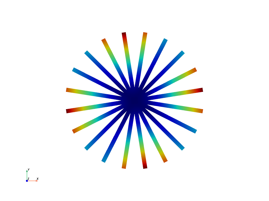
Plot First Bend for Nodal Diameter 2#
Note how you can clearly see two nodal lines for this mode shape since it’s nodal diameter 2.
result.plot_nodal_displacement(
    12, cpos="xy", cmap="jet", show_scalar_bar=False, add_text=False
)
Animate First Bend for Nodal Diameter 2#
Let’s end this example by animating mode 12, which corresponds to first bend for the 2nd nodal diameter of this example model.
_ = result.animate_nodal_displacement(
    12,
    displacement_factor=2e-4,
    movie_filename="traveling_wave12.gif",
    n_frames=30,
    off_screen=True,
    loop=False,
    add_text=False,
    show_scalar_bar=False,
    cmap="jet",
)
Total running time of the script: (0 minutes 32.811 seconds)