Note
Go to the end to download the full example code.
Path Operations within PyMAPDL and MAPDL#
This tutorial shows how you can use pyansys and MAPDL to interpolate along a path for stress. This shows some advanced features of the pyvista module to perform the interpolation.
First, start MAPDL as a service and disable all but error messages.
import matplotlib.pyplot as plt
import numpy as np
import pyvista as pv

from ansys.mapdl.core import launch_mapdl

mapdl = launch_mapdl(loglevel="ERROR")
MAPDL: Solve a Beam with a Non-Uniform Load#
Create a beam, apply a load, and solve for the static solution.
# beam dimensions
width_ = 0.5
height_ = 2
length_ = 10
# simple 3D beam
mapdl.clear()
mapdl.prep7()
mapdl.mp("EX", 1, 70000)
mapdl.mp("NUXY", 1, 0.3)
mapdl.csys(0)
mapdl.blc4(0, 0, 0.5, 2, length_)
mapdl.et(1, "SOLID186")
mapdl.type(1)
mapdl.keyopt(1, 2, 1)
mapdl.desize("", 100)
mapdl.vmesh("ALL")
# mapdl.eplot()
# fixed constraint
mapdl.nsel("s", "loc", "z", 0)
mapdl.d("all", "ux", 0)
mapdl.d("all", "uy", 0)
mapdl.d("all", "uz", 0)
# arbitrary non-uniform load
mapdl.nsel("s", "loc", "z", length_)
mapdl.f("all", "fz", 1)
mapdl.f("all", "fy", 10)
mapdl.nsel("r", "loc", "y", 0)
mapdl.f("all", "fx", 10)
mapdl.allsel()
mapdl.run("/solu")
sol_output = mapdl.solve()
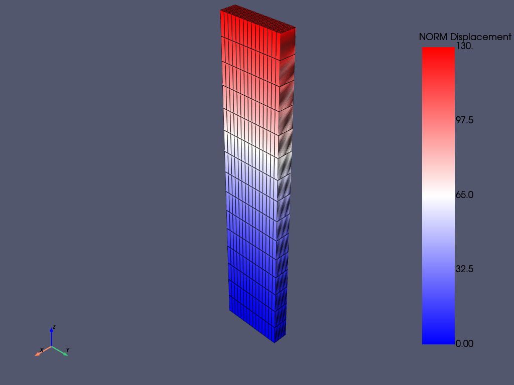
# plot the normalized global displacement
mapdl.post_processing.plot_nodal_displacement(lighting=False, show_edges=True)
Post-Processing - MAPDL Path Operation#
Compute the stress along a path within MAPDL and convert the result to a numpy array
mapdl.post1()
mapdl.set(1, 1)
# mapdl.plesol("s", "int")

# path definition
pl_end = (0.5 * width_, height_, 0.5 * length_)
pl_start = (0.5 * width_, 0, 0.5 * length_)

mapdl.run("width_ = %f" % width_)
mapdl.run("height_ = %f" % height_)
mapdl.run("length_ = %f" % length_)

mapdl.run("pl_end = node(0.5*width_, height_, 0.5*length_)")
mapdl.run("pl_start = node(0.5*width_, 0, 0.5*length_)")
mapdl.path("my_path", 2, ndiv=100)
mapdl.ppath(1, "pl_start")
mapdl.ppath(2, "pl_end")

# mapping components of interest to path.
mapdl.pdef("Sx_my_path", "s", "x")
mapdl.pdef("Sy_my_path", "s", "y")
mapdl.pdef("Sz_my_path", "s", "z")
mapdl.pdef("Sxy_my_path", "s", "xy")
mapdl.pdef("Syz_my_path", "s", "yz")
mapdl.pdef("Szx_my_path", "s", "xz")

# Extract the path results from MAPDL and send to a numpy array
nsigfig = 10
mapdl.header("OFF", "OFF", "OFF", "OFF", "OFF", "OFF")
mapdl.format("", "E", nsigfig + 9, nsigfig)
mapdl.page(1e9, "", -1, 240)

path_out = mapdl.prpath(
    "Sx_my_path",
    "Sy_my_path",
    "Sz_my_path",
    "Sxy_my_path",
    "Syz_my_path",
    "Szx_my_path",
)
table = np.genfromtxt(path_out.splitlines()[1:])
print("Numpy Array from MAPDL Shape:", table.shape)
Numpy Array from MAPDL Shape: (101, 7)
Comparing with Path Operation Within pyvista#
The same path operation can be performed within pyvista by saving
the resulting stress and storing within the underlying UnstructuredGrid
Take note that there is slight piece-wise behavior in both MAPDL’s and VTK’s interpoltion methods (both of which result in nearly identical interpolations). The underlying algorithm of VTK is:
The `vtkProbeFilter`, once it finds the cell containing a query
point, uses the cell's interpolation functions to perform the
interpolate / compute the point attributes.
# same thing in pyvista
rst = mapdl.result
nnum, stress = rst.nodal_stress(0)
# get SYZ stress
stress_yz = stress[:, 5]
# Assign the YZ stress to the underlying grid within the result instance.
# For this example, NAN values must be replaced with 0 for the
# interpolation to succeed
stress_yz[np.isnan(stress_yz)] = 0
rst.grid["Stress YZ"] = stress_yz
# Create a line and sample over it
line = pv.Line(pl_start, pl_end, resolution=100)
out = line.sample(rst.grid) # bug where the interpolation must be run twice
out = line.sample(rst.grid)
# Note: We could have used a spline (or really, any dataset), and
# interpolated over it instead of a simple line.
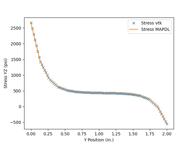
# plot the interpolated stress from VTK and MAPDL
plt.plot(out.points[:, 1], out["Stress YZ"], "x", label="Stress vtk")
plt.plot(table[:, 0], table[:, 6], label="Stress MAPDL")
plt.legend()
plt.xlabel("Y Position (in.)")
plt.ylabel("Stress YZ (psi)")
plt.show()
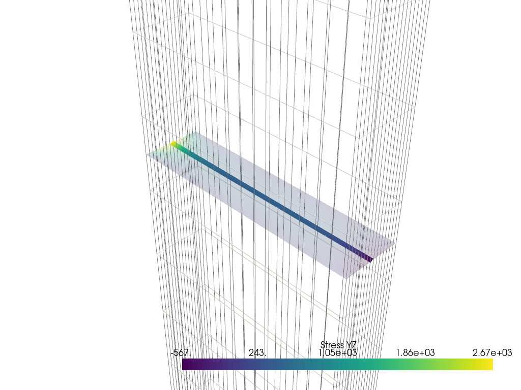
2D Slice Interpolation#
Take a 2D slice along the beam and plot it alongside the stress at the line.
Note that this slice occurs between the edge nodes of this beam, necessitating interpolation as stress/strain is (in general) extrapolated to the edge nodes of ANSYS FEMs.
stress_slice = rst.grid.slice("z", pl_start)

# can plot this individually
# stress_slice.plot(scalars=stress_slice['Stress YZ'],
#                   scalar_bar_args={'title': 'Stress YZ'})

# good camera position (determined manually using pl.camera_position)
cpos = [(3.2, 4, 8), (0.25, 1.0, 5.0), (0.0, 0.0, 1.0)]
max_ = np.max((out["Stress YZ"].max(), stress_slice["Stress YZ"].max()))
min_ = np.min((out["Stress YZ"].min(), stress_slice["Stress YZ"].min()))
clim = [min_, max_]

pl = pv.Plotter()
pl.add_mesh(
    out,
    scalars=out["Stress YZ"],
    line_width=10,
    clim=clim,
    scalar_bar_args={"title": "Stress YZ"},
)
pl.add_mesh(
    stress_slice,
    scalars="Stress YZ",
    opacity=0.25,
    clim=clim,
    show_scalar_bar=False,
)
pl.add_mesh(rst.grid, color="w", style="wireframe", show_scalar_bar=False)
pl.camera_position = cpos
_ = pl.show()
Stop mapdl#
mapdl.exit()
Total running time of the script: (0 minutes 3.839 seconds)