Note
Go to the end to download the full example code.
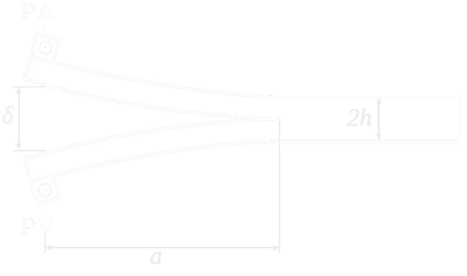
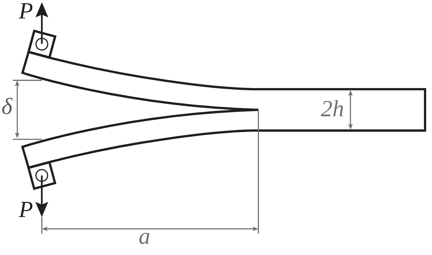
Static simulation of double cantilever beam test via cohesive elements#
This example is a classic double cantilever beam test commonly used to study mode I interfacial delamination of composite plates.
Description#
Objective#
This example shows how to use PyMAPDL to simulate delamination in composite materials. PyDPF modules are also used for the postprocessing of the results.
Problem figure#
Procedure#
Launch the MAPDL instance.
Set up the model.
Solve the model.
Plot results using PyMAPDL.
Plot results using PyDPF.
Plot reaction force.
Additional packages#
These additional packages are imported for use: * - Matplotlib for plotting * - Pandas for data analysis and manipulation
Start MAPDL as a service#
This example begins by importing the required packages and then launching Ansys Mechanical APDL.
import os
import tempfile

from ansys.dpf import core as dpf
import matplotlib.pyplot as plt
import numpy as np
import pyvista as pv

from ansys.mapdl.core import launch_mapdl

# Start MAPDL as a service
mapdl = launch_mapdl()
print(mapdl)
Mapdl
-----
PyMAPDL Version:     0.73.2
Interface:           grpc
Product:             Ansys Mechanical Enterprise
MAPDL Version:       25.2
Running on:          localhost
                     (127.0.0.1)
Set geometrical inputs#
Set geometrical inputs for the model.
Set up the model#
Set up the model by choosing the units system and the
element types for the simulations. Because a fully 3D approach
is chosen for this example, SOLID186 elements are used for meshing volumes, and
TARGE170 and CONTA174 are used for modelling cohesive elements in between contact
surfaces.
Define material parameters#
Composite plates are modelled using homogeneous linear elastic orthotropic properties, whereas a bilinear cohesive law is used for cohesive elements.
# Enter the preprocessor and define the unit system
mapdl.prep7()
mapdl.units("mpa")

# Define SOLID185, TARGE170, and CONTA174 elements, along with the element size
mapdl.et(1, 185)
mapdl.et(2, 170)
mapdl.et(3, 174)
mapdl.esize(10.0)

# Define material properties for the composite plates
mapdl.mp("ex", 1, 61340)
mapdl.mp("dens", 1, 1.42e-09)
mapdl.mp("nuxy", 1, 0.1)

# Define the bilinear cohesive law
mapdl.mp("mu", 2, 0)
mapdl.tb("czm", 2, 1, "", "bili")
mapdl.tbtemp(25.0)
mapdl.tbdata(1, 50.0, 0.5, 50, 0.5, 0.01, 2)
DATA FOR  CZM  TABLE FOR MATERIAL   2 AT TEMPERATURE=  25.0000
 LOC=  1 5.00000e+01     5.00000e-01     5.00000e+01     5.00000e-01     1.00000e-02     2.00000e+00
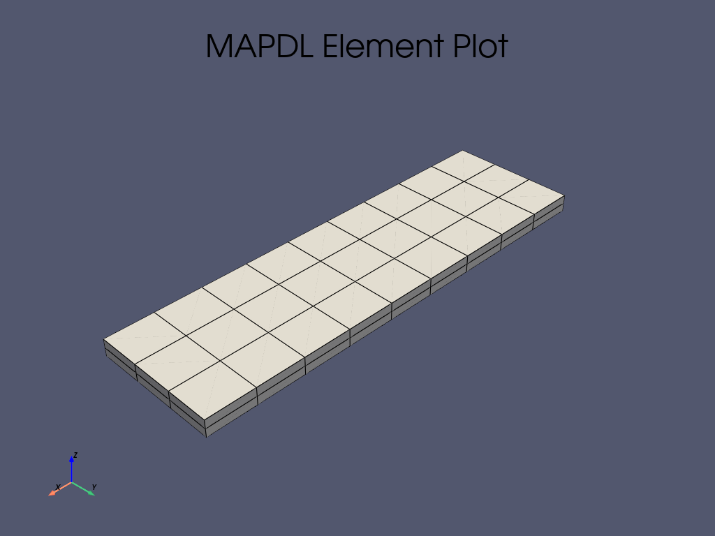
Create the geometry in the model and meshing#
The two plates are generated as two parallelepipeds. Composite material properties and the three-dimensional elements are then assigned.
# Generate the two composite plates
vnum0 = mapdl.block(0.0, length + pre_crack, 0.0, width, 0.0, height)
vnum1 = mapdl.block(0.0, length + pre_crack, 0.0, width, height, 2 * height)

# Assign material properties and element type
mapdl.mat(1)
mapdl.type(1)

# performing the meshing
mapdl.vmesh(vnum0)
mapdl.vmesh(vnum1)

mapdl.esel("all")
mapdl.eplot()
Generate cohesive elements in between the contact surfaces#
The generation of cohesive elements is the most delicate part of the
modelling approach. First, the two contact surfaces are identified
and defined as a components (in this case cm_1 and cm_2 respectively).
Then, the real constants for the CONTA174 and TARGE170 elements and
their key options are set to capture the correct behavior. Descriptions for each
of these parameters can be found in the Ansys element documentation.
Finally, elements are generated on top of the respective surfaces cm_1 and
cm_2.
# Identify the two touching areas and assign them to components
mapdl.allsel()
mapdl.asel("s", "loc", "z", 1.7)
mapdl.asel("r", vmin=mapdl.geometry.anum[0])
mapdl.nsla("r", 1)
mapdl.nsel("r", "loc", "x", pre_crack, length + pre_crack + eps)
mapdl.components["cm_1"] = "node"

mapdl.allsel()
mapdl.asel("s", "loc", "z", 1.7)
mapdl.asel("r", vmin=mapdl.geometry.anum[1])
mapdl.nsla("r", 1)
mapdl.nsel("r", "loc", "x", pre_crack, length + pre_crack + eps)
mapdl.components["cm_2"] = "node"

# Identify all the elements before generation of TARGE170 elements
mapdl.allsel()
mapdl.components["_elemcm"] = "elem"
mapdl.mat(2)

# Assign real constants and key options
mapdl.r(3, "", "", 1.0, 0.1, 0, "")
mapdl.rmore("", "", 1.0e20, 0.0, 1.0, "")
mapdl.rmore(0.0, 0.0, 1.0, "", 1.0, 0.5)
mapdl.rmore(0.0, 1.0, 1.0, 0.0, "", 1.0)
mapdl.rmore("", "", "", "", "", 1.0)
mapdl.keyopt(3, 4, 0)
mapdl.keyopt(3, 5, 0)
mapdl.keyopt(3, 7, 0)
mapdl.keyopt(3, 8, 0)
mapdl.keyopt(3, 9, 0)
mapdl.keyopt(3, 10, 0)
mapdl.keyopt(3, 11, 0)
mapdl.keyopt(3, 12, 3)
mapdl.keyopt(3, 14, 0)
mapdl.keyopt(3, 18, 0)
mapdl.keyopt(3, 2, 0)
mapdl.keyopt(2, 5, 0)

# Generate TARGE170 elements on top of cm_1
mapdl.nsel("s", "", "", "cm_1")
mapdl.components["_target"] = "node"
mapdl.type(2)
mapdl.esln("s", 0)
mapdl.esurf()

# Generate CONTA174 elements on top of cm_2
mapdl.cmsel("s", "_elemcm")
mapdl.nsel("s", "", "", "cm_2")
mapdl.components["_contact"] = "node"
mapdl.type(3)
mapdl.esln("s", 0)
mapdl.esurf()
GENERATE ELEMENTS ON SURFACE DEFINED BY SELECTED NODES
  TYPE=        3  REAL=        1  MATERIAL=        2  ESYS=    0

 NUMBER OF ELEMENTS GENERATED=         21
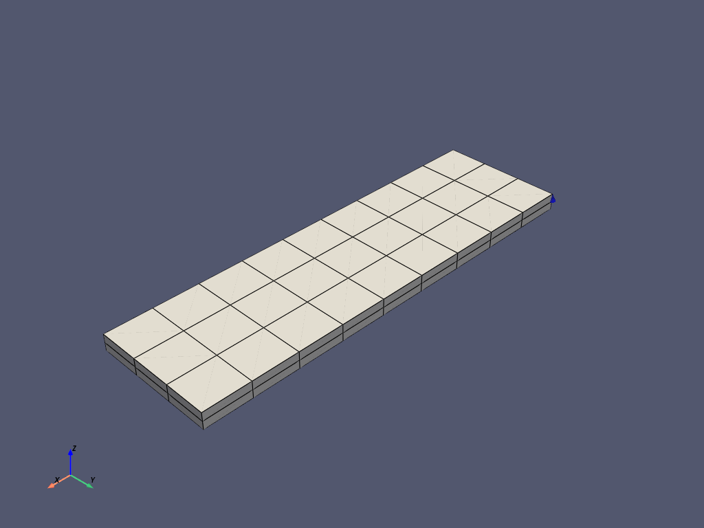
Generate boundary conditions#
Assign boundary conditions to replicate the real test conditions. One end of the two
composite plates is fixed against translation along the x, y, and z axis. On the
opposite side of the plate, displacement conditions are applied to
simulate the interfacial crack opening. These conditions are applied to the
top and bottom nodes corresponding to the geometrical edges located
respectively at these (x, y, z) coordinates:, (0.0, `y`, 0.0) and (0.0, `y`, 3.4).
Two different components are assigned to these sets of nodes for a faster
identification of the nodes bearing reaction forces.
# Apply the two displacement conditions
mapdl.allsel()
mapdl.nsel(type_="s", item="loc", comp="x", vmin=0.0, vmax=0.0)
mapdl.nsel(type_="r", item="loc", comp="z", vmin=2 * height, vmax=2 * height)
mapdl.d(node="all", lab="uz", value=d)
mapdl.components["top_nod"] = "node"

mapdl.allsel()
mapdl.nsel(type_="s", item="loc", comp="x", vmin=0.0, vmax=0.0)
mapdl.nsel(type_="r", item="loc", comp="z", vmin=0.0, vmax=0.0)
mapdl.d(node="all", lab="uz", value=-10)
mapdl.components["bot_nod"] = "node"

mapdl.allsel()
mapdl.eplot(
    plot_bc=True,
    bc_glyph_size=3,
    title="Applied displacements",
    cpos=[-1, 1, 1],
)

# Apply the fix condition
mapdl.allsel()
mapdl.nsel(
    type_="s",
    item="loc",
    comp="x",
    vmin=length + pre_crack,
    vmax=length + pre_crack,
)
mapdl.d(node="all", lab="ux", value=0.0)
mapdl.d(node="all", lab="uy", value=0.0)
mapdl.d(node="all", lab="uz", value=0.0)


mapdl.allsel()
mapdl.eplot(
    plot_bc=True,
    bc_glyph_size=3,
    title="Fixed boundary condition",
)
Solve the non-linear static analysis#
Run a non-linear static analysis. To have smooth crack opening progression and facilitate convergency for the static solver, request 100 substeps.
# Enter the solution processor and define the analysis settings
mapdl.allsel()
mapdl.finish()
mapdl.solution()
mapdl.antype("static")

# Activate non-linear geometry
mapdl.nlgeom("on")

# Request substeps
mapdl.autots(key="on")
mapdl.nsubst(nsbstp=100, nsbmx=100, nsbmn=100)
mapdl.kbc(key=0)
mapdl.outres("all", "all")

# Solve
output = mapdl.solve()
Postprocessing#
Use PyMAPDL and PyDPF for postprocessing.
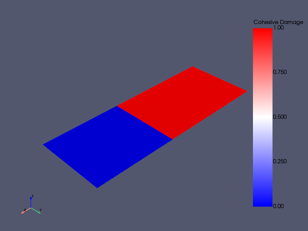
Postprocess results using PyMAPDL#
This section shows how to use PyMAPDL to postprocess results. Because
measuring the delamination length is important, plot the cohesive damage parameter.
Although the damage parameter is an element parameter, the result is
provided in terms of a nodal result. Thus, the result for just one of
the four-noded cohesive element NMISC = 70 is presented.
The result for the other nodes are present at NMISC = 71,72,73.
You can retrieve the actual damage parameter nodal values from the
solved model in form of a table (or an array).
# Enter the postprocessor
mapdl.post1()

# Select the substep
mapdl.set(1, 100)

# Select ``CONTA174`` elements
mapdl.allsel()
mapdl.esel("s", "ename", "", 174)

# Plot the element values
mapdl.post_processing.plot_element_values(
    "nmisc", 70, scalar_bar_args={"title": "Cohesive Damage"}
)

# Extract the nodal values of the damage parameter
mapdl.allsel()
mapdl.esel("s", "ename", "", 174)
mapdl.etable("damage", "nmisc", 70)

damage_df = mapdl.pretab("damage").to_dataframe()
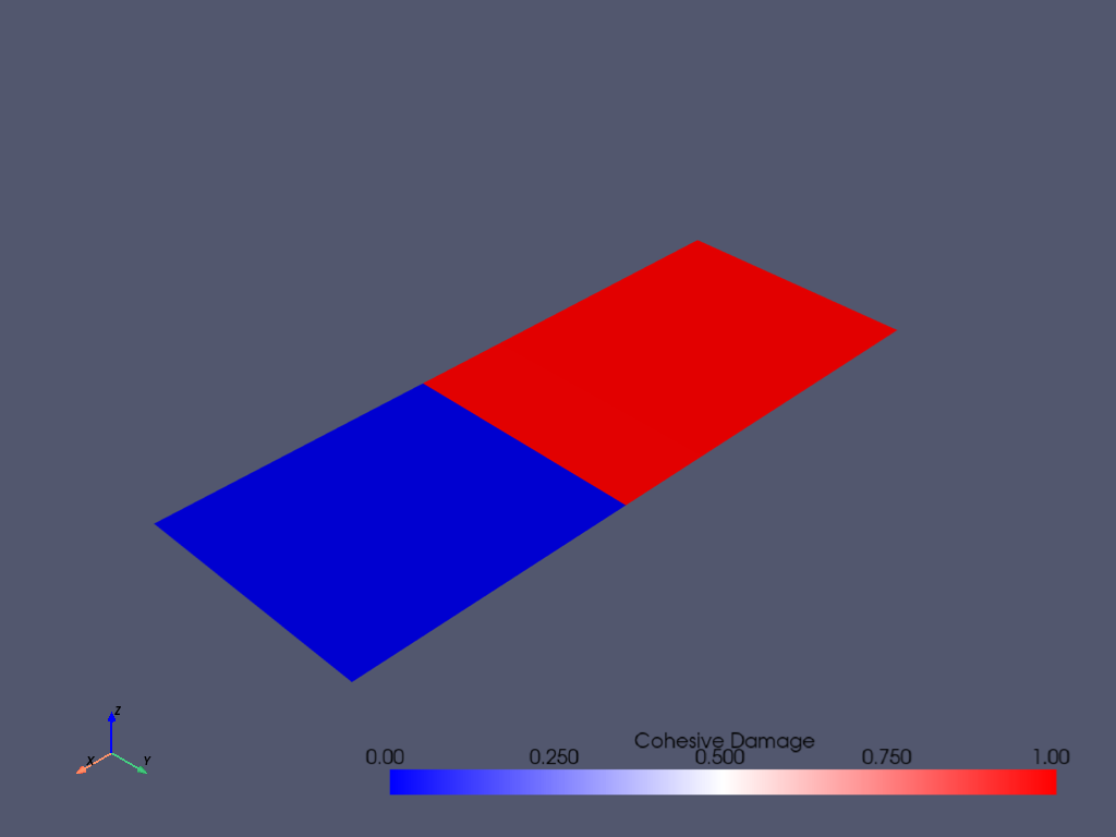
Postprocessing results using PyDPF#
Use PyDPF to visualize the crack opening throughout the simulation as an animation.
temp_directory = tempfile.gettempdir()
rst_path = mapdl.download_result(temp_directory)


server_is_local = "DPF_PORT" not in os.environ

if server_is_local:
    # Local server
    dpf_server = dpf.server.start_local_server()
    path_source = rst_path

else:
    # Remote server
    dpf_server = dpf.server.connect_to_server(port=int(os.environ["DPF_PORT"]))
    path_source = dpf.upload_file_in_tmp_folder(rst_path)
    os.remove(rst_path)  # Delete local copy

# Building the model
model = dpf.Model(path_source, dpf_server)

# Get the mesh of the whole model
meshed_region = model.metadata.meshed_region

# Get the mesh of the cohesive elements
mesh_scoping_cohesive = dpf.mesh_scoping_factory.named_selection_scoping(
    "CM_1", model=model
)

result_mesh = dpf.operators.mesh.from_scoping(
    scoping=mesh_scoping_cohesive, inclusive=0, mesh=meshed_region
).eval()

# Get the coordinates field for each mesh
mesh_field = meshed_region.field_of_properties(dpf.common.nodal_properties.coordinates)
mesh_field_cohesive = result_mesh.field_of_properties(
    dpf.common.nodal_properties.coordinates
)

# Get the index of the NMISC results
nmisc_index = 70

# Generate the damage result operator
data_src = dpf.DataSources(path_source)
dam_op = dpf.operators.result.nmisc(data_sources=data_src, item_index=70)

# Generate the displacement operator
disp_op = model.results.displacement()

# Create sum operators to compute the updated coordinates at step n
add_op = dpf.operators.math.add(fieldA=mesh_field)
add_op_cohesive = dpf.operators.math.add(fieldA=mesh_field_cohesive)

# Instantiate a PyVista plotter and start the creation of a GIF
plotter = pv.Plotter(notebook=False, off_screen=True)
plotter.open_gif("dcb.gif")

# Add the beam mesh to the scene
mesh_beam = meshed_region.grid
plotter.add_mesh(
    mesh_beam,
    lighting=False,
    show_edges=True,
    scalar_bar_args={"title": "Cohesive Damage"},
    clim=[0, 1],
    opacity=0.3,
)


# Add the contact mesh to the scene
mesh_contact = result_mesh.grid
damage_scalars_name = "Cohesive Damage"
mesh_contact.cell_data[damage_scalars_name] = np.zeros(mesh_contact.n_cells)
mesh_contact.set_active_scalars(damage_scalars_name, preference="cell")
plotter.add_mesh(
    mesh_contact,
    opacity=0.9,
    scalar_bar_args={"title": "Cohesive Damage"},
    clim=[0, 1],
    scalars=damage_scalars_name,
)
for i in range(1, 100):
    # Get displacements
    disp = model.results.displacement(time_scoping=i).eval()
    # Getting the updated coordinates
    add_op.inputs.fieldB.connect(disp[0])
    disp_result = add_op.outputs.field()
    # Get displacements for the cohesive layer
    disp = model.results.displacement(
        time_scoping=i, mesh_scoping=mesh_scoping_cohesive
    ).eval()
    # Get the updated coordinates for the cohesive layer
    add_op_cohesive.inputs.fieldB.connect(disp[0])
    disp_cohesive = add_op_cohesive.outputs.field()
    # Get the damage field
    dam_op.inputs.time_scoping([i])
    cohesive_damage = dam_op.outputs.fields_container()[0]
    # Update coordinates and scalars

    mesh_beam.points = disp_result.data
    mesh_contact.points = disp_cohesive.data
    mesh_contact.cell_data[damage_scalars_name][:] = cohesive_damage.data
    plotter.write_frame()

plotter.close()
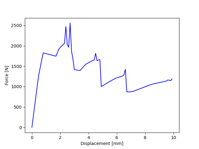
Plot the reaction force at the bottom nodes
mesh_scoping = model.metadata.named_selection("BOT_NOD")
f_tot = []
d_tot = []
for i in range(100):
    force_eval = model.results.element_nodal_forces(
        time_scoping=i, mesh_scoping=mesh_scoping
    ).eval()
    force = force_eval[0].data
    f_tot += [np.sum(force[:, 2])]
    d = abs(
        model.results.displacement(time_scoping=i, mesh_scoping=mesh_scoping)
        .eval()[0]
        .data[0]
    )
    d_tot += [d[2]]

d_tot[0] = 0
f_tot[0] = 0

fig, ax = plt.subplots()

plt.plot(d_tot, f_tot, "b")
plt.ylabel("Force [N]")
plt.xlabel("Displacement [mm]")
plt.show()
Animate results using PyDPF with .animate() method#
Use PyDPF method FieldsContainer.animate() to visualize the crack opening throughout the simulation as
an animation.
disp = model.results.displacement.on_all_time_freqs.eval()
camera_pos = disp.animate(
    scale_factor=1.0,
    save_as="dcb_animate.gif",
    return_cpos=True,
    show_axes=True,
)
Exit MAPDL
mapdl.exit()
Total running time of the script: (1 minutes 6.129 seconds)