Note
Go to the end to download the full example code.
Dynamic Load Effect on a Supported Thick Plate#
This example demonstrates how to perform a random vibration analysis using PyMAPDL.
This example is based on the ANSYS Verification Manual, problem 203 (VM203).
Description#
A simply-supported thick square plate of length L, thickness t, and mass per unit area m is subject to random uniform pressure power spectral density. Determine the peak one-sigma displacement at undamped natural frequency.
A frequency range of 1.0 Hz to 80 Hz is used as an approximation of the white noise PSD forcing function frequency. The PSD curve is a constant $$(1E6 N/m^2)^2 / Hz$$.
The model is solved using SHELL281 elements and generic materials.
Import modules#
import matplotlib.pyplot as plt
from tabulate import tabulate

from ansys.mapdl.core import launch_mapdl

mapdl = launch_mapdl()

mapdl.clear()
mapdl.prep7()
mapdl.units("mks")
MKS UNITS SPECIFIED FOR INTERNAL
  LENGTH        (l)  = METER (M)
  MASS          (M)  = KILOGRAM (KG)
  TIME          (t)  = SECOND (SEC)
  TEMPERATURE   (T)  = CELSIUS (C)
  TOFFSET            = 273.0
  CHARGE        (Q)  = COULOMB
  FORCE         (f)  = NEWTON (N) (KG-M/SEC2)
  HEAT               = JOULE (N-M)

  PRESSURE           = PASCAL (NEWTON/M**2)
  ENERGY        (W)  = JOULE (N-M)
  POWER         (P)  = WATT (N-M/SEC)
  CURRENT       (i)  = AMPERE (COULOMBS/SEC)
  CAPACITANCE   (C)  = FARAD
  INDUCTANCE    (L)  = HENRY
  MAGNETIC FLUX      = WEBER
  RESISTANCE    (R)  = OHM
  ELECTRIC POTENTIAL = VOLT

 INPUT  UNITS ARE ALSO SET TO MKS
Parameters#
Loading parameters
LOAD_PRES = -1e6
DAMPING_RATIO = 0.02
Set up the FE model#
Set the element type to SHELL281, which is a 3D structural high-order shell element.
Shell Section ID= 1 Number of layers= 1 Total Thickness= 1.000000
Set material properties#
Units are in the international unit system.
MATERIAL 1 DENS = 8000.000
Create geometry#
Create the model geometry.
GENERATE       4 TOTAL SETS OF ELEMENTS WITH NODE INCREMENT OF        40
   SET IS SELECTED ELEMENTS IN RANGE         1 TO         4 IN STEPS OF       1

 MAXIMUM ELEMENT NUMBER=        16
Loads and boundary conditions#
Define loads and boundary conditions.
Apply a uniform pressure load of 1,000,000 N/m^2
mapdl.sfe("ALL", "", "PRES", "", LOAD_PRES)
SPECIFIED SURFACE LOAD PRES FOR ALL SELECTED ELEMENTS  LKEY =  1   KVAL = 1
     VALUES =   -0.10000E+07   -0.10000E+07   -0.10000E+07   -0.10000E+07
Apply constraints UX, UY, ROTZ DOFs all fixed
mapdl.d("ALL", "UX", 0, "", "", "", "UY", "ROTZ")
SPECIFIED CONSTRAINT UX   FOR SELECTED NODES            1 TO         169 BY           1
 REAL=  0.00000000       IMAG=  0.00000000
 ADDITIONAL DOFS=  UY    ROTZ
Simply supported on the four corners
mapdl.d(1, "UZ", 0, 0, 9, 1, "ROTX")
mapdl.d(161, "UZ", 0, 0, 169, 1, "ROTX")
mapdl.d(1, "UZ", 0, 0, 161, 20, "ROTY")
mapdl.d(9, "UZ", 0, 0, 169, 20, "ROTY")
SPECIFIED CONSTRAINT UZ   FOR SELECTED NODES            9 TO         169 BY          20
 REAL=  0.00000000       IMAG=  0.00000000
 ADDITIONAL DOFS=  ROTY
Solve the model#
Solve the modal analysis using the PCG Lanczos solver to find and expand the first two modes of the model.
FINISH SOLUTION PROCESSING


 ***** ROUTINE COMPLETED *****  CP =         0.000
PSD Spectrum analysis#
Now let’s perform PSD spectrum analysis using the two solved modes:
mapdl.slashsolu()
mapdl.antype("SPECTR")
mapdl.spopt("PSD", n_modes, "ON")
USE PSD RESPONSE SPECTRUM
  USE THE FIRST    2 MODES FROM THE MODAL ANALYSIS
  INCLUDE STRESS RESPONSES IN THE CALCULATIONS
  PSD INTEGRATION WILL BE PERFORMED IN CLOSED FORM
Define the PSD spectrum
mapdl.psdunit(1, "PRES")
PSD TYPE FOR TABLE NUMBER 1 IS PRES
Applying proportional damping
mapdl.dmprat(DAMPING_RATIO)
DAMPING RATIO = 0.0200
PSD frequency value table 1 to 80 Hz
PSD VALUES (DIAGONAL) FOR TABLE  1
   PSDVAL =    1.0000        1.0000
Define the PSD load vector generated at modal analysis
mapdl.sfedele("ALL", "", "PRES")
mapdl.lvscale(1)
mapdl.pfact(1, "NODE")
COMPUTE PARTICIPATION FACTORS FOR TABLE   1
  FOR NODAL EXCITATION

 *****  MAPDL PFACT    COMMAND  *****

 *** SELECTION OF ELEMENT TECHNOLOGIES FOR APPLICABLE ELEMENTS ***
                ---GIVE SUGGESTIONS ONLY---

 ELEMENT TYPE         1 IS SHELL281. IT IS ASSOCIATED WITH ELASTOPLASTIC
 MATERIALS ONLY. KEYOPT(8)=2 IS SUGGESTED.


   *****MAPDL VERIFICATION RUN ONLY*****
     DO NOT USE RESULTS FOR PRODUCTION

                       S O L U T I O N   O P T I O N S

   PROBLEM DIMENSIONALITY. . . . . . . . . . . . .3-D
   DEGREES OF FREEDOM. . . . . . UX   UY   UZ   ROTX ROTY ROTZ
   ANALYSIS TYPE . . . . . . . . . . . . . . . . .SPECTRUM
      SPECTRUM TYPE. . . . . . . . . . . . . . . .PSD
   NUMBER OF MODES TO BE USED. . . . . . . . . . .     2
   ELEMENT RESULTS CALCULATION . . . . . . . . . .ON
   GLOBALLY ASSEMBLED MATRIX . . . . . . . . . . .SYMMETRIC

 *** NOTE ***                            CP =       0.000   TIME= 00:00:00
 The conditions for direct assembly have been met.  No .emat or .erot
 files will be produced.

                      L O A D   S T E P   O P T I O N S

   LOAD STEP NUMBER. . . . . . . . . . . . . . . .     2
   MODAL DAMPING RATIO . . . . . . . . . . . . . . 0.20000E-01
   PRINT OUTPUT CONTROLS . . . . . . . . . . . . .NO PRINTOUT
   DATABASE OUTPUT CONTROLS. . . . . . . . . . . .ALL DATA WRITTEN

   *****MAPDL VERIFICATION RUN ONLY*****
     DO NOT USE RESULTS FOR PRODUCTION


  ***** PARTICIPATION FACTORS FOR NODAL EXCITATION *****    TABLE NO.    1

  MODE   VALUE      MODE   VALUE      MODE   VALUE      MODE   VALUE

    1  -90096.        2   2.4549
Write out the displacement result
mapdl.psdres("DISP", "REL")
# set for PSD mode combination method
mapdl.psdcom()
mapdl.solve()

mapdl.finish()
FINISH SOLUTION PROCESSING


 ***** ROUTINE COMPLETED *****  CP =         0.000
Post-processing#
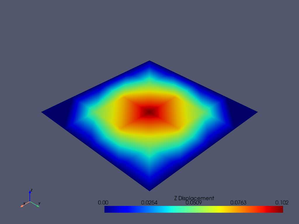
Now we can plot the results of the one-sigma displacement solution. We will plot the Z displacement of the nodes.
mapdl.post1()
# One Sigma Displacement Solution Results
mapdl.set(3, 1)
mapdl.post_processing.plot_nodal_displacement("Z", cmap="jet", cpos="iso")
mapdl.finish()
EXIT THE MAPDL POST1 DATABASE PROCESSOR


 ***** ROUTINE COMPLETED *****  CP =         0.000
Use post26 to capture then plot the response psd and the max value
number_frequencies = 2
mapdl.post26()
mapdl.store("PSD", number_frequencies)

node85_uz = mapdl.nsol(2, 85, "U", "Z")
rpsduz = mapdl.rpsd(3, 2, "", 1, 2)
While you can use the extrem command to get the maximum and minimum values:
print(mapdl.extrem(2, 3))
POST26 SUMMARY OF VARIABLE EXTREME VALUES
 VARI TYPE    IDENTIFIERS   NAME     MINIMUM    AT TIME    MAXIMUM   AT TIME

   2 NSOL    85 UZ        UZ       -0.1269E-007  0.000      0.1017       0.000
   3 OPER     3 RPSD      3          0.000       0.000      0.3595E-002  0.000
You can also use Numpy methods to find the max value of the response psd.
+---------------------------------+------------+-------------+
|                                 |  Maximum   |   Minimum   |
+=================================+============+=============+
|       Z-displacement on node 85 | 1.0171e-01 | -1.2690e-08 |
+---------------------------------+------------+-------------+
| Response power spectral density | 3.5954e-03 | 0.0000e+00  |
+---------------------------------+------------+-------------+
To get the maximum value of the response psd you can use the get_value ( wrapper of *GET) method with the EXTREM option:
Pmax = mapdl.get_value("VARI", 3, "EXTREM", "VMAX")
However, you can also use the numpy methods here as well:
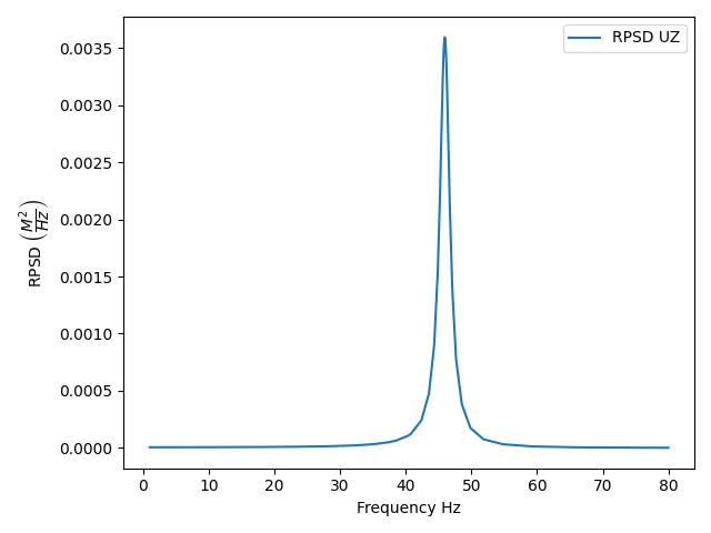
You can plot the response psd using MAPDL methods:
# Setting up the PSD plot with MAPDL
mapdl.axlab("X", "Frequency (Hz)")
mapdl.axlab("Y", "RPSD (M**2/Hz)")
mapdl.yrange(ymin="0", ymax="0.004")
mapdl.xrange(xmin="0", xmax="80")
mapdl.gropt(lab="LOGY", key="ON")

mapdl.xvar(0)  # Plot against time/frequency
mapdl.plvar(3)  # Plot variable set 3 (RPSD)
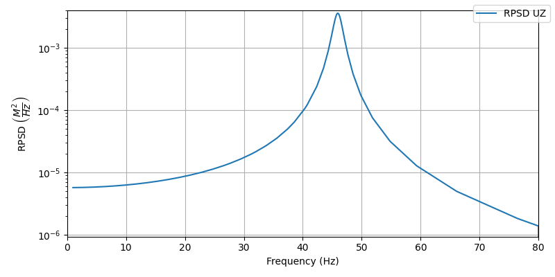
or use matplotlib:
freqs = mapdl.vget("FREQS", 1)

# Remove the last two values as they are zero
fig, ax = plt.subplots(figsize=(8, 4))

ax.plot(freqs, rpsduz, label="RPSD UZ")

ax.set_yscale("log")
ax.set_xlabel("Frequency (Hz)")
ax.set_ylabel(r"RPSD $\left( \dfrac{M^2}{Hz}\right)$")
ax.set_xlim((0, 80))
ax.set_ylim((0, 0.004))
ax.grid()

fig.legend()

fig.tight_layout()
fig.show()
Compare and print results to manual values
+------------------------------+------------+--------------+---------+
|                              |     Manual |   Calculated |   Ratio |
+==============================+============+==============+=========+
| Frequency (Hz)               | 45.9       |   45.9596    | 1.0013  |
+------------------------------+------------+--------------+---------+
| Peak Deflection PSD (m^2/Hz) |  0.0034018 |    0.0035954 | 1.05691 |
+------------------------------+------------+--------------+---------+
Exit MAPDL
mapdl.exit()
Total running time of the script: (0 minutes 1.734 seconds)